Neural Processing from the Ground Up
Have you ever wondered how Apple’s Neural Engine or Google’s first-generation Tensor Processing Unit (TPU v1) works under the hood? This post introduces the concepts that underlie neural processing, and explores how different neural network accelerators realise those concepts in silicon.
My hope is that this post leaves you with an understanding of the concepts, and an appreciation for the capabilities (and limitations) of the hardware. This will help you to better optimise models for deployment on embedded devices.
Code
This post includes several Python code snippets. Full examples can be found in my neural-processing repo on GitHub.
Contents
- Terminology
- Matrix Multiplication
- Tensors
- Convolutional Filters
- Architecture
- Systolic Arrays
- Software Stack
- Model Compatibility
- Wrap Up
Terminology
As with many technologies, the terminology around neural network accelerators has been muddied by marketing. Let’s see if we can clear things up a bit.
A Neural Processing Unit (NPU) is any processor designed to accelerate neural network workloads. These are often found in embedded devices, where they are designed specifically for inference - i.e. running an already-trained model. However, this does not preclude NPUs being deployed in larger systems, or being used for training. NPUs vary greatly in capabilities, and some are very capable of training and fine-tuning models.
Tensor Processing Unit (TPU) is Google’s name for a family of neural network accelerators. A TPU is a kind of NPU, rather than a mutually exclusive architecture. Different processor designs accelerate tensor operations in different ways. In smaller devices, lower-precision arithmetic may be used to fit more computation and data into a given transistor and power budget. Larger devices may support higher precision, while offering high throughput with a much larger number of cores.
This post will focus on Google’s TPU, Apple’s Neural Engine (ANE), and Rockchip NPUs. The same concepts should apply to other neural processors. Unless I mention otherwise, the TPU hardware discussed below is TPU v1, and TPU v2 will be used for comparison.
Google TPU
Google’s TPU is noteworthy as an early example of dedicated neural-network accelerators deployed at data-centre scale. First used internally in 2015 (before being announced publicly in 2016), it helped establish specialised matrix-processing hardware as a practical solution for large-scale machine learning.
The first generation of TPUs targeted inference, using 8-bit integer arithmetic arranged in a systolic array - think of this as a grid of processing elements, or cells, where data is passed between between neighbouring cells. Systolic arrays are not a new idea, dating back to 1978, but their application to large-scale neural-networks was a significant step forward.
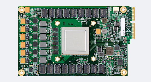
Google’s first Tensor Processing Unit (TPU v1) on a printed circuit board.
Image credit: An in-depth look at Google’s first Tensor Processing Unit (TPU v1)
Google has continued to innovate aggressively on the TPU architecture. TPU v2, the second-generation TPU announced in 2017, supported training as well as inference, with floating-point arithmetic and interconnects linking devices into TPU pods. These are high-powered devices intended for server deployment:
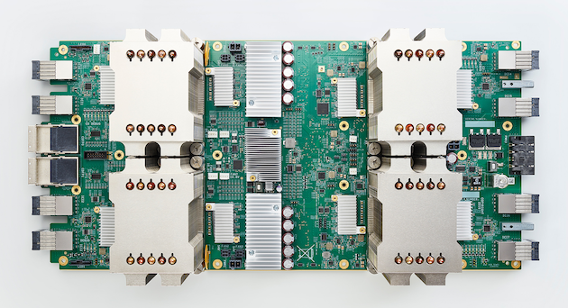
Google’s second-generation Tensor Processing Unit (TPU v2).
Image credit: Build and train machine learning models on TPU v2
Apple Neural Engine
Not long after, Apple introduced the Apple Neural Engine (ANE) in the A11 Bionic chip in 2017. This chip feature in iPhone 8/Plus and iPhone X. Apple’s Neural Engine is a dedicated, highly parallel tensor accelerator optimised for inference.
The goal was to run neural networks locally within a phone’s power budget. Like other neural processing units, it uses specialised hardware to accelerate computationally intensive operations such as convolutions and matrix multiplication, rather than executing these operations as general-purpose CPU instructions.
The original two-core design handled up to 600 billion operations per second, supporting features such as Face ID on the iPhone X. When the M1 was introduced in 2020, it included a 16-core Neural Engine rated at 11 TOPS (trillion operations per second).
Mac and iOS applications typically access Neural Engine cores through Core ML, which can distribute a model’s computation across the CPU, GPU, and Neural Engine. This is an example of heterogeneous computing.
Rockchip NPU
In 2018, Rockchip announced its first fully integrated NPU, the RK3399Pro. This was Rockchip’s first processor combining a CPU, GPU, and dedicated NPU. It focuses on inference, using models that have been specially quantised and calibrated to fit within the constraints of the NPU. Its affordability made it popular in development boards such as the Khadas Edge 1:
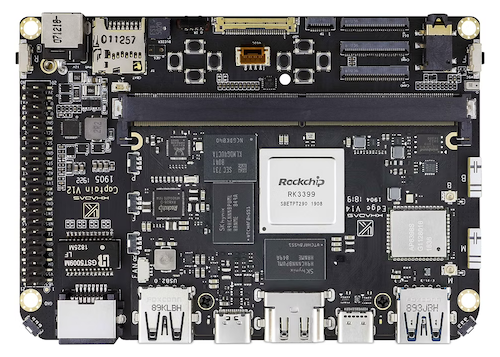
Image credit: Khadas
The RK3399Pro was fundamentally a convolution-oriented tensor accelerator. The design leveraged parallel multiply-accumulate (MAC) units that can also perform matrix multiplication. This makes it well suited to visual processing using CNNs, while also supporting other neural network architectures.
Later generations (such as RK3588) expanded support for a broader range of neural network architectures, including transformers and language models, while retaining the same fundamental emphasis on efficient, parallel tensor computation.
A common theme across all architectures is matrix multiplication, which we’ll discuss next.
Matrix Multiplication
A matrix multiplication takes as input two matrices, of size $M \times K$ and $K \times N$, and produces an output matrix of size $M \times N$. The shared dimension $K$ collapses in the middle:
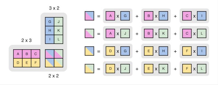
We see this all the time in neural networks, where a weight matrix is multiplied with a vector or matrix derived from user input.
A naive CPU implementation can be written as three nested loops:
# 1. Outer loop: Iterates through each ROW of Matrix A
for m in range(M):
    # 2. Middle loop: Iterates through each COLUMN of Matrix B
    for n in range(N):
        # 3. Inner loop: Accumulate products to calculate dot product
        for k in range(K):
            C[m][n] += A[m][k] * B[k][n]
These nested loops perform a total of $M \times K \times N$ multiply-accumulate steps, so the arithmetic work is $O(MKN)$. If all three dimensions are equal to $n$ (square matrices), this simplifies to $O(n^3)$. The number of operations can become large for larger dimensions. Now we’ll see how a hardware implementation can do this more efficiently.
Multiply-Accumulate (MAC) Units
The example above shows us that a multiply-accumulate (MAC) is a fundamental operation performed in neural networks. We simply multiply two numbers, then add the product to an accumulator. Performing many MAC operations in parallel is crucial to achieving competitive performance in an NPU.
Parallel execution is achieved using an array of MAC units. Each MAC unit is a processing element that calculates the product of two numbers, then adds that product to an local accumulator. Each MAC operation is triggered by the rising edge of a clock signal, which is one of the MAC unit’s inputs.
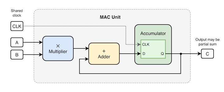
Once we have a sufficient number of MAC units, we can combine them to implement a Matrix Multiplier.
Scale matters here! TPU v1’s Matrix Multiply Unit (MXU) contains 65,536 8-bit integer MAC units, arranged as a 256x256 array. For comparison, some GPUs have thousands of 32-bit floating-point arithmetic units. This gives the TPU a distinct advantage when performing large matrix multiplications.
A 4x4 Matrix Multiplier
To better understand how a Matrix Multiply Unit works, we can construct our own little multiplier. Ours will support 4x4 square matrices, so $M = K = N = 4$. This would consist of 16 MAC units:
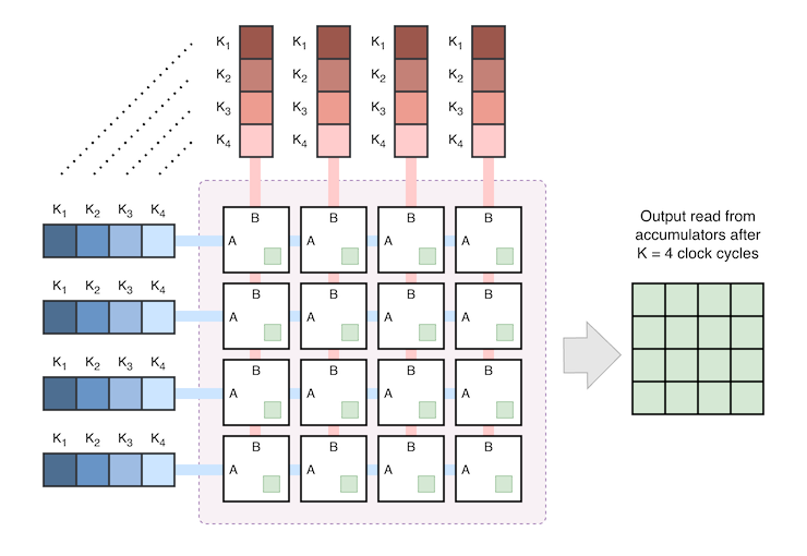
When implemented in hardware, the MAC units operate in parallel. Two of the nested loops are eliminated, leaving just one loop for the inner dimension $K$. In Python, this would look like:
multiplier = MatMul_4x4()

for k in range(4):
    multiplier.tick(k)
One advantage of this design is that K can scale freely. Each iteration of K corresponds to a clock cycle on real hardware. This means $M = N = 4$, while $K$ is free to change.
Tiling
If we would also like to scale $M$ and $N$, then we need to implement a tiling strategy.
To keep this manageable, let’s assume that we only have a 2x2 matrix multiplier (e.g. MatMul_2x2 instead of MatMul_4x4).
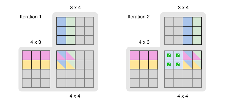
To handle output matrices larger than 2x2, we can divide the output matrix into regular 2x2 tiles. To calculate an output tile, we multiply the corresponding input tiles and accumulate their results across the shared dimension ($K$). This gives us the flexibility to handle larger matrices, at the cost of reintroducing two nested loops:
# Initialise a matrix multiplier for this tile
matmul = Matmul_2x2()

# Tiles are each 2 x 2 in size
for row_offset in range(0, M, 2):
    for col_offset in range(0, N, 2):
        # Reset the accumulators
        matmul.clear()

        # Perform K accumulation steps, one per cycle in this simplified model.
        for k in range(K):
            multiplier.tick(k, row_offset, col_offset)

        # Write the tile's at most 4 output values into C.
        copy(matmul.result(), C, row_offset, col_offset);
Here’s what this looks like if we step through execution, where each iteration computes one 2x2 tile. The first two iterations complete the first row of 2x2 tiles:
The third and fourth iteration complete the second row of 2x2 tiles:
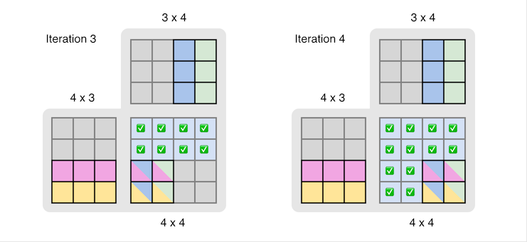
Note: For simplicity, we’ve ignored data transfer and synchronisation requiremetns. A major challenge in implementing a tiled matrix multiplier in hardware is ensuring that data is available when a tile is ready to be computed.
Complexity
How does this translate to hardware?
Our toy 2×2 matrix multiplier has four MAC units, one for each output in a 2×2 tile. Each tile performs $K$ accumulation steps, and the number of tiles is $\lceil M/2 \rceil \times \lceil N/2 \rceil$. So the ideal number of compute cycles is $K \times \lceil M/2 \rceil \times \lceil N/2 \rceil$, assuming one MAC operation per unit per clock cycle.
Despite this, the computational complexity is still $O(MKN)$. Although the 2×2 tiled hardware can reduce the ideal compute cycles relative to a single MAC unit, this is a constant factor reduction. Tiling necessarily has two outer loops.
Furthermore, the speed-up depends on how well the MAC array is kept supplied with data and on other overheads. Writing the output tile to memory takes $O(MN)$ work. And for dimensions not divisible by two, edge tiles will contain fewer valid outputs or require padding
Tensors
Tensors come up frequently in the implementation of neural networks.
A tensor is a generalisation of a multidimensional array, applicable even to scalars (singular values). A scalar has zero axes, a vector has one, and a matrix has two. Arrays with three or more axes are generally just called “tensors”, although the term is valid for smaller dimensions too. The number of axes is sometimes called the tensor’s rank.
I always enjoy this visualisation:
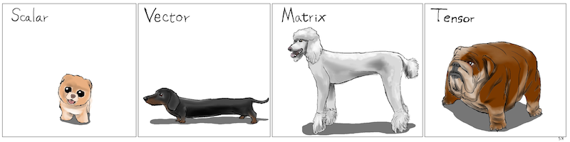
Linear Dogs, illustrated by Karl Stratos.
As an example, an image is commonly represented with three axes: [height, width, channels]. Similarly, a batch of images has four: [batch, height, width, channels].
What we’ll see below is how matrix multiplication can be used to implement common tensor operations. We can reshape and combine two tensors by multiplying values and summing over a shared axis, an operation called a contraction.
Tensor Multiplication
Consider a neural-network layer that transforms each token’s 512 input features into 2,048 output features. Suppose we process 32 sequences, each containing 128 tokens. The same set of weights are used for every token, in every sequence.
Ignoring the bias and activation for now, the input shapes are:
Input X:    [32, 128, 512]           batch, token, input feature (k)
Weights W:           [512, 2048]                   input feature (k), output feature
The input is a tensor of rank three. And the weights are rank two. The output is 2048 features for each token, of each sequence, which is rank three:
Output Y: [32, 128, 2048] batch, token, output feature
Note that the input-feature axis (k) is summed away. The batch and token axes remain, and every token uses the same weights. Each output can be calculated as:
Y[b, s, o] = sum over k of X[b, s, k] * W[k, o]
Reshaping
Naively, this would be implemented as three nested loops. There’s another trick we can use, which is to reshape the input tensor. This allows us to flatten out the dimensions, while preserving the data layout in memory. We start by reshaping the input, so that the first two dimensions are combined into one (32 x 128 = 4096):
[32, 128, 512] -> [4096, 512]
Reshaping is non-destructive. Combining these axes changes how we index the data, not the underlying data. Crucially, it allows us to express the operation using regular matrix multiplication:
[4096, 512] × [512, 2048] → [4096, 2048]
Finally we reshape the output to restore the rank:
[4096, 2048] → [32, 128, 2048]
Arithmetic Operations
This illustrates how higher-dimensional tensor operations can be implemented through ordinary matrix multiplications. You shouldn’t need to do this manually - a driver or framework often takes responsibility for reshaping, tiling, and scheduling tensor operations as matrix multiplications.
Even with this reshaping trick, tensor operations often need a very large number of multiply-accumulate (MAC) operations. The example above requires 4096 × 512 × 2048 = 4,294,967,296 MAC operations. Counting a multiplication and an addition separately gives about 8.6 billion arithmetic operations.
That’s matrix multiplication and tensors. The last concept we’ll introduce is convolution.
Convolutional Filters
A convolutional filter is a small set of learned weights that spans the input channels and moves across the spatial dimensions of the input tensor. At each position, the filter calculates a weighted sum of the values in the receptive area:
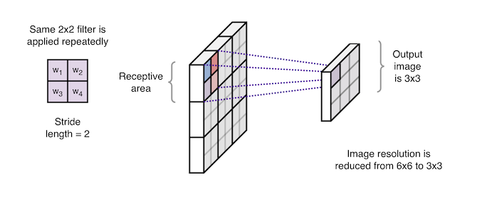
The set of weights is often called a ‘kernel’.
At each output position, convolution computes a dot product between the kernel weights and the corresponding region of the input tensor. Neighbouring regions can overlap, so the same input values may contribute to several output positions.
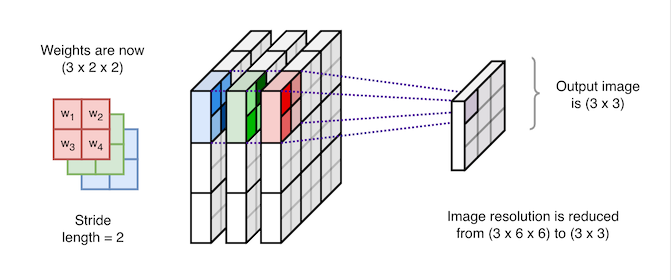
Input Channels
Convolutional filters are not limited to two dimensional inputs. It’s common for a convolution filter to be applied to three- or four-dimensional inputs, such as images. A kernel can be stacked to separate red, green, and blue input channels:
Strides and Padding
To fully specify a convolution, we also need to consider its stride and padding. The stride determines how far the filter moves between positions. For example, a stride of one checks every adjacent position, while a stride of two skips every second position, and so on.
Padding adds values around the input’s edges. This allows a filter to get more exposure to border pixels and, along with stride length, allows more control over the output size.
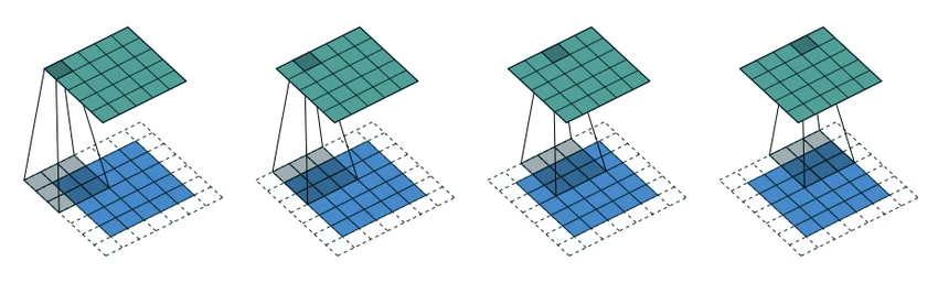
An example of a 3x3 filter applied with stride and padding = 1.
Image credit: Text to Image Synthesis Using Generative Adversarial Networks
Convolutional Layers
In neural networks, you will typically see Convolutional Filters stacked together in a single “Convolutional Layer”. Each filter represents a separate output channel, with its own learnable weights:
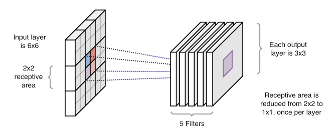
A convolutional layer is often characterised by the number and shape of trainable weights. What’s important here is that the shape of the weights is determined by the number of input channels and output channels, as well as the size, stride and padding of the kernel.
Consider a convolutional layer with:
- 64 input channels
- 128 output channels
- 3×3 kernel
This requires $64 \times 128 \times 3 \times 3 = 73,728$ learned weights (excluding biases). This means each spatial output position involves 73,728 MAC operations, when applied to all 128 output channels.
Although this is a relatively modest number of trainable weights, the number of MAC operations grows rapidly for larger inputs. The important thing to take away from this is that, due to the rate at which computations scale, neural processors often include specialised support for convolutional filters.
Architecture
Now that we’ve reviewed the math, it’s time to discuss hardware architecture. We necessarily simplify the building blocks to help explain concepts that apply to NPU architectures and the TPU v1 discussed here.
We start with how memory is structured in a neural processor.
Memory Hierarchy
A key design goal for a neural processor is keep data close to where it is needed in compute cores. Failing to do so means that operations are delayed waiting for data to be loaded from system memory, or worse, from disk storage.
The following chart shows how quickly these numbers grow in a typical NPU memory hierarchy:
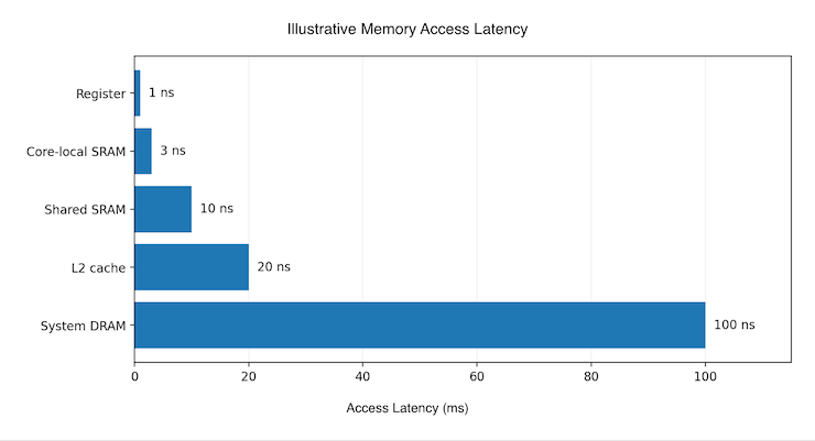
As you move from the top to the bottom of the memory hierarchy, storage capacity increases, but so does latency. At the extremes, a system DRAM access may be 100 times slower than register access on an NPU core. Within a neural processor, you will often find L1 / L2 caches, on-chip shared memory (known as the scratchpad), and SRAM local to each compute core:
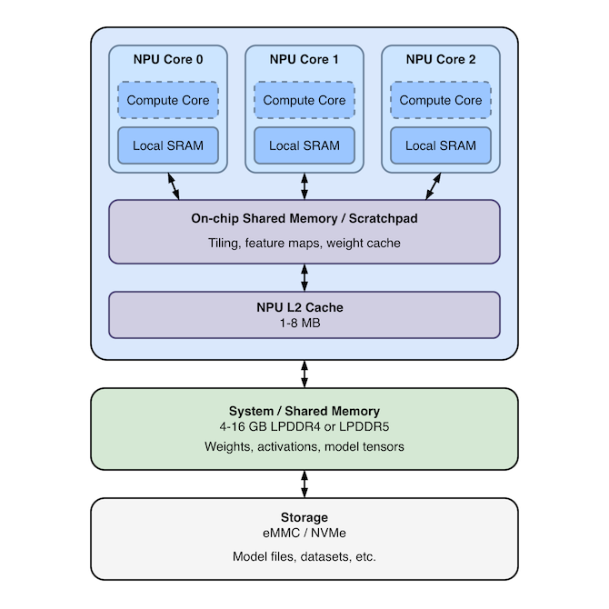
Here’s what this looks like at every level:
| Memory Level | Description | Purpose |
|---|---|---|
| Registers | Inside each compute core, immediately adjacent to the MAC and tensor units. | Hold operands and partial sums during computation. |
| Core-local SRAM | Fast working memory dedicated to individual compute cores. | Stores small tiles of activations, weights, and intermediate results. |
| Shared SRAM | On-chip memory accessible by multiple compute units, often implemented as a scratchpad. | Enables data sharing and reuse of weights or activations without repeatedly accessing DRAM. |
| L2 Cache | On-chip cache for data read from system DRAM. | Reduces repeated data transfers over the system bus. |
| System DRAM | Main system memory with substantially greater capacity than on-chip memory. | Holds model weights, input tensors, and larger intermediate tensors that cannot fit on-chip. |
| Persistent Storage | Non-volatile storage, such as eMMC, flash, or SSD. | Stores model files before they are loaded into memory. |
Direct Memory Access
The separation of system and on-chip memory introduces its own challenges, as data needs to be transferred between system and on-chip memory banks. A traditional solution is to use a Direct Memory Access (DMA) controller, which manages data transfers between components in a system:
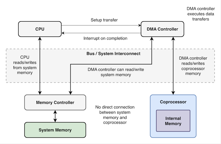
A major advantage of DMA is that, after a transfer request is issued by the CPU, the DMA controller can transfer data without the CPU being involved. The CPU (or device driver) needs to map buffers, configure the transfer, handle completion or errors, and synchronize data access. But the transfer itself is asynchronous.
An NPU typically uses a variation of this architecture, in which there is a dedicated on-chip DMA engine. Although the NPU has access to system memory, the DMA engine is responsible for transferring input tiles, weights, and results between system memory and on-chip memory:
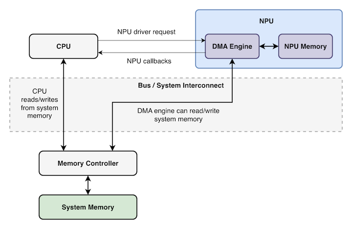
The CPU is still minimally involved - it submits work through an NPU driver, which sets up buffers and commands for the NPU. The DMA engine can then perform the requested transfers, while the CPU handles synchronization and any follow-up work.
Many neural processors will also use double or triple buffering to overlap data movement with computation. For example, the NPU can operate on one tile in local SRAM while the DMA engine loads the next tile into another buffer. This is, of course, subject to available bandwidth.
Systolic Arrays
Systolic arrays are an architectural approach commonly seen in VLSI (Very-large-scale integration) circuit design. This approach allows a circuit to be implemented as a uniform grid of processing elements, with data flowing through the grid on each rising edge of a clock:
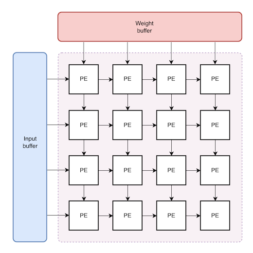
This is the core idea behind Google’s TPU v1, which used a 256 × 256 systolic array consisting of 65,536 8-bit multiply-accumulate units. The arrays shown here are much smaller, so we can follow how data moves through them. They illustrate the same basic pattern at a much smaller scale than the full TPU v1 design.
Processing Elements
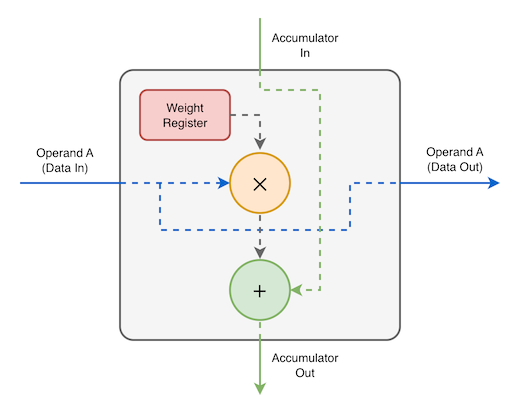
Each cell in a systolic array is known as a processing element (PE). Like the MAC units we saw earlier, individual PEs execute MAC operations and accumulate a result. The difference is that a PE must also pass its inputs to neighbouring cells in the next clock cycle:
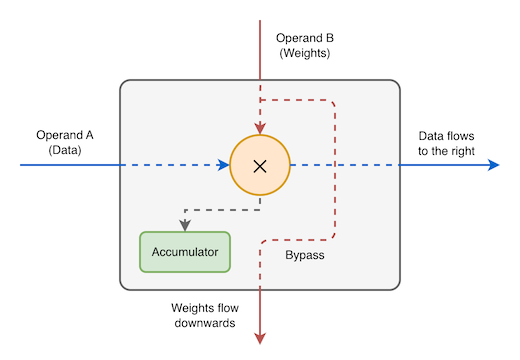
This particular PE uses an output-stationary architecture. For matrix multiplication there are two common architectures: Output-stationary and weight-stationary. We’ll start by looking at an output-stationary array.
Output-Stationary Arrays
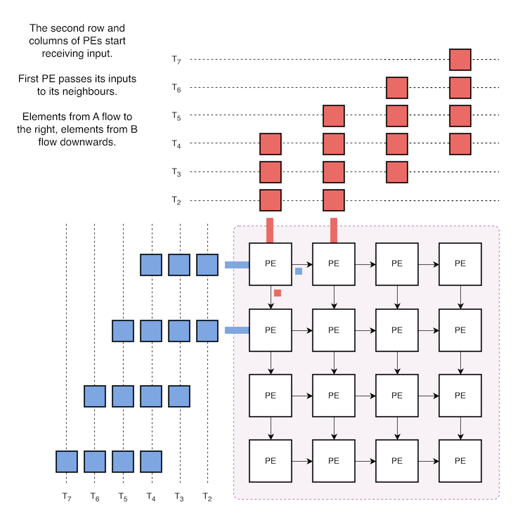
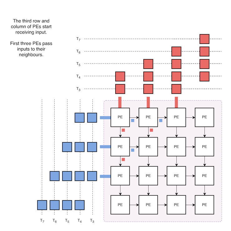
The key characteristic of an output-stationary array is that each PE in the array has its own accumulator register. In the diagrams below, data inputs flow in from the left, and weights from in from above. This might be a little confusing at first, because the weights matrix is flipped vertically:
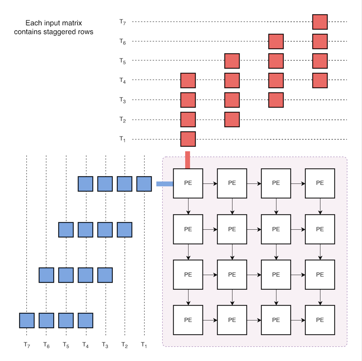
In the systolic array above, we can see that at $T = 1$, only the top-left PE is ready to process its inputs. On the first clock cycle, that PE will calculate the product of those two inputs, and add it to its internal accumulator.
When we progress to $T = 2$, the top-left PE passes those same inputs to its neighbours. If we focus on the second PE in the first row, we can see that it receives input A at the same time that input B becomes available from above:
We can see how this continues at $T = 3$. In this case, PE(1,1) is the first element to receive its inputs exclusively from neighbouring cells:
That’s output-stationary arrays in a nutshell.
Weight-Stationary Arrays
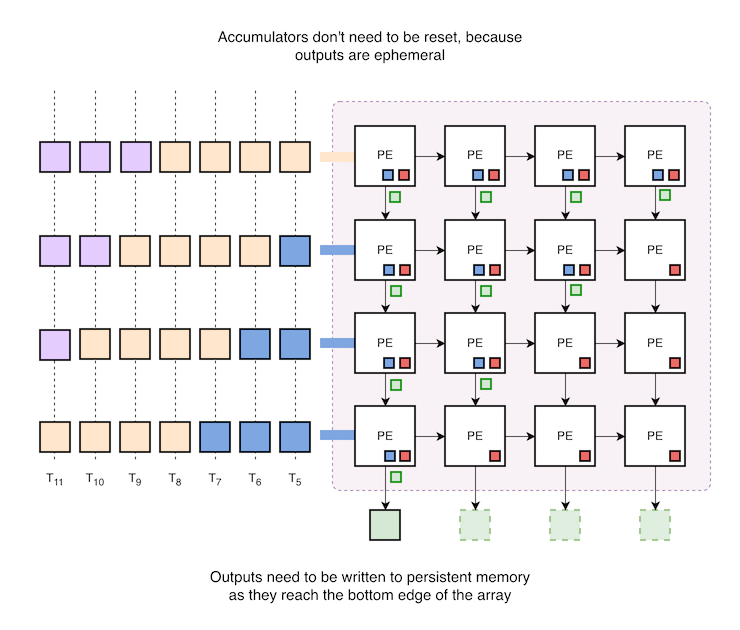
Our other choice is a Weight-Stationary architecture, in which the weights are loaded just once. Inputs still flow from left to right, but now its the accumulators that flow downwards through each processing element:
TPU v1 is a practical example of a weight-stationary systolic design. Weights are pre-loaded into the array, then reused as input values flow through it. Outputs exit from the bottom of the array. This is well suited to streaming data through the same model weights.
This is illustrated below, where the first input is blue, and the second input is orange:
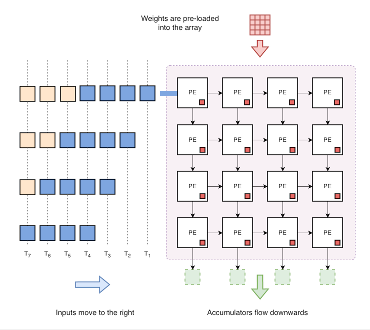
A drawback of this approach is that every time a column output hits the bottom edge of the grid, it must be written out to memory. This causes heavy write traffic when processing small batch sizes.
We begin to see this at $T = 5$:
Software Stack
There are multiple ways to configure and control an accelerator. This is true not just for neural processors, but for any kind of accelerator you might find in a PC or embedded device. Google, Apple and Rockchip all take different approaches here, ranging from dedicated instruction sets to register-based configuration and control.
Instruction Sets
TPU v1 used a CISC-style architecture, featuring an instruction set specialised for operations relevant to neural networks. This includes instructions to transfer data between system memory and on-chip SRAM, perform matrix multiplications, and apply activation functions. Instructions are issued to TPU v1 primarily by Google’s XLA runtime, which is responsible for mapping a model graph onto the hardware. Once a program is loaded, execution can proceed independently. Later TPU variants differ, and their details are beyond the scope of this overview.
Register Control
Rockchip NPUs sit at the opposite end of this spectrum - the NPU is configured primarily through hardware registers, and these must be updated continuously to drive the chip. Rockchip’s runtime and driver stack is responsible for doing this. The runtime is actively involved in scheduling operations, transferring data to/from system memory, and configuring fixed function pipelines.
Dedicated Firmware
Apple’s Neural Engine is architecturally closer to the Rockchip NPU than to Google’s TPU v1. It features a dedicated execution controller, which has its own firmware. This means there are effectively two different configuration and control interfaces to consider: the actual program executed by the accelerator and the command protocol used to communicate with its firmware.
Heterogeneous Computing
Heterogeneous computing refers to systems that use more than one kind of processor or core to perform a task. Apple and Google both support heterogeneous compute, albeit at the framework level.
For Apple devices, when a model is loaded by CoreML, the framework can decide whether it runs on the CPU, GPU or Neural Engine. It can also choose whether all or part of a model graph should execute on a Neural Engine core, and only then does it hand over control to the Neural Engine firmware.
Google’s TPU software ecosystem supports heterogeneous computing via high-level frameworks such as JAX. Computations are expressed independently of the underlying hardware, leaving compilers such as XLA to optimise and translate operations for CPUs, GPUs, and Google’s TPU family. This describes the broader software ecosystem, not TPU v1 hardware specifically.
Model Compatibility
The model produced during training is often incompatible with a target NPU architecture.
Precision
TPU v1 used 8-bit integer arithmetic. Later TPU generations support floating-point formats such as Float16 and BFloat16 (Brain Floating Point Format). More generally, processors may use lower precision to improve performance and reduce memory footprint:
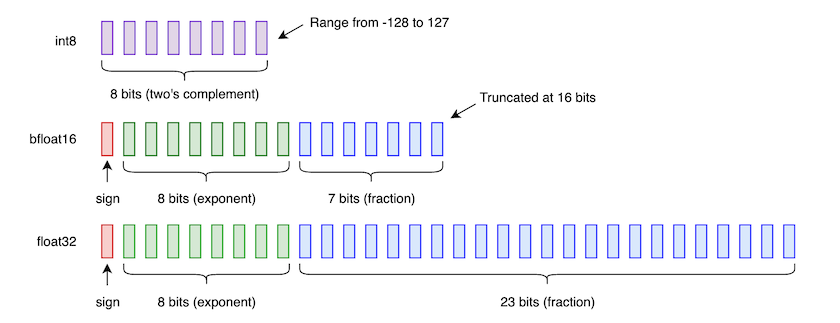
A comparison of different levels of numeric precision, showing how they differ in capacity.
Models trained at higher precision will need their weights and activations quantised. This is likely to have a negative impact on model accuracy, which is something you need to keep an eye out for.
In other cases, it may be impossible to run a model on an NPU due to certain layers or operations not being supported by the processor architecture. For example, models that rely on dynamic graph operations are not well supported on Rockchip NPUs. Therefore, deploying on an embedded device may end up being non-trivial.
Conversion
Each architecture provides its own tooling and workflows for converting a model into format that is compatible with the hardware:
CoreML
Apple’s Core ML Tools converts models from frameworks such as PyTorch and TensorFlow into Core ML format. Once converted, the model can be run on Neural Engine, or the CPU or GPU. Conversion is performed in Python:
import torch
import coremltools as ct

# Prepare the PyTorch model
model = MyNet().eval()
example = torch.randn(1, 3, 224, 224)

# Export the computation graph
exported = torch.export.export(model, (example,))

# Convert to Core ML
mlmodel = ct.convert(
    exported,
    inputs=[
        ct.ImageType(
            name="image",
            shape=example.shape,
            color_layout=ct.colorlayout.RGB,
            scale=1 / 255.0,
        )
    ],
    minimum_deployment_target=ct.target.iOS17,
)

# Add metadata and save
mlmodel.short_description = "Image classifier v1.3"
mlmodel.save("Classifier.mlpackage")
RKNN-Toolkit2
Rockchip’s RKNN-Toolkit2 converts supported models into RKNN format on a development computer. Rockchip also provides RKLLM for converting large language models into a format supported by the NPU. This has matured in recent years, and now supports a wide range of transformer models.
Conversion is also performed in Python:
from rknn.api import RKNN

rknn = RKNN(verbose=True)

try:
    # Configure preprocessing and target hardware
    rknn.config(
        target_platform="rk3588",
        mean_values=[[0, 0, 0]],
        std_values=[[255, 255, 255]],
        quantized_dtype="asymmetric_quantized-8",
    )

    # Load the ONNX model
    assert rknn.load_onnx(model="classifier.onnx") == 0

    # Build and quantize using representative samples
    assert rknn.build(
        do_quantization=True,
        dataset="calibration.txt",
    ) == 0

    # Export the compiled model
    assert rknn.export_rknn("classifier_rk3588.rknn") == 0

finally:
    rknn.release()
Google Cloud
Google Cloud TPU platforms support frameworks such as JAX and PyTorch, which use XLA to translate model operations into hardware-specific instructions. Unlike the Apple and Rockchip tooling described above, the model is not exported into a proprietary deployment format.
Compilation
Google’s approach highlights a difference between model conversion and model compilation. Conversion changes a model from a framework’s representation into a format accepted by a deployment tool or runtime. For example, Core ML Tools converts a model into Core ML format, while RKNN-Toolkit2 converts a supported model into RKNN format. Conversion may also involve quantisation.
Compilation takes the model’s computational graph and turns it into an executable format for a specific target device. The compiler can optimise and combine operations, choose how to schedule them, and generate instructions or device-specific representation. On Google Cloud, this is handled primarily by XLA, which supports ahead-of-time or just-in-time compilation.
This distinction between conversion and compilation is useful, but the steps can overlap. Conversion may involve compilation, and a runtime may compile a graph when it is loaded or first executed.
Wrap Up
We’ve covered a wide range of topics in this post: matrix multiplication, tiling, systolic arrays, convolutional filters, tensors, different kinds of processor cores, and NPU software stacks.
My hope is that you now have an appreciation of the differences between common neural processor architectures, and how you might use that knowledge to inform your model and hardware choices in the future.
References
- Google’s TPU architecture overview describes the broader TPU family; the bfloat16 explanation concerns later TPU generations, not TPU v1.
- Apple’s Core ML documentation describes model conversion with Core ML Tools, application integration, and execution across CPU, GPU, and Neural Engine.
- Apple’s Core ML Tools provides tools to convert machine learning models from third-party libraries to the Core ML format.
- Google’s LiteRT overview describes its portable on-device model format and conversion/runtime workflow. Cloud TPU runtime documentation covers the broader Cloud TPU software ecosystem, not TPU v1 specifically.
- Rockchip’s RKNN-Toolkit2 project describes model conversion and deployment through RKNN runtime interfaces.
- Rockchip’s RK3588 brief datasheet shows this system context.
Honourable Mentions
I’ve focused on TPU v1, Apple’s Neural Engine, and Rockchip’s NPUs above, because those are the architectures I’m most familiar with. However, it would be foolish to overlook other significant players in this space:
- Qualcomm Hexagon is the NPU used in Snapdragon platforms, accelerating on-device inference in smartphones and PCs.
- Intel AI Boost is the integrated NPU in Intel Core Ultra processors. It targets sustained AI workloads at low power, complementing the CPU and GPU.
- AMD XDNA is the NPU architecture behind Ryzen AI. It uses a tiled array of AI Engine processors, with local memory and connections that allow data to flow between tiles.
- Arm Ethos-U85 is an NPU design that chip makers can integrate into their own SoCs. It targets embedded and IoT applications, including convolutional and transformer networks.
Also worth a mention is IBM’s TrueNorth, described in 2014. TrueNorth explored a different, brain-inspired approach.