Machine Translation at the Edge: Part 2
In the previous post, we introduced the machine translation problem and worked through the fundamentals of the MarianNMT framework. For this installment, we’ve set ourselves a goal to port Marian to the Rockchip NPU. More precisely, we want to download a pretrained MarianMT model from Hugging Face, convert it to Rockchip’s RKNN format, then perform inference directly on the Rockchip NPU - all using Python!
Throughout this journey, we discuss issues such as quantization, input padding and layer compatibility. For those wanting more detail, the complete source code for this project can be found on GitHub. This includes a native C++ implementation too!
Contents
- Part 1 Recap
- Preflight
- Converting to ONNX
- Converting to RKNN
- Inference Engine
- Decoding Strategies
- Benchmarks
- Next Steps
- References
Part 1 Recap
When it comes to Machine Translation, there are several well-established models we can choose from. After exploring a few options, we ultimately decided to focus on Marian Transformer-based models. These models have seen adoption in industry and are available for a wide range of language pairs. Marian is also simple enough that if we wanted to support transformer-based models trained using another toolkit, such as Sockeye or OpenNMT, many of the same techniques would apply.
Let’s visit what “Marian” actually means, starting with MarianNMT.
MarianNMT
MarianNMT is a pure C++ machine learning toolkit, specialised for training Neural Machine Translation (NMT) models. MarianNMT can be compiled to run on the CPU, or with GPU-acceleration using CUDA. Although it can be used to train a range of different machine translation models (e.g. LSTMs and Seq2Seq models) it is most commonly used to train Transformer models.
MarianNMT includes an efficient inference engine, also written in C++. This is highly portable, but is not written in a way that enables adoption of the RKNN API. If we tried to cross-compile Marian for Rockchip devices, processing would still happen on the CPU, which is not what we want.
So we’ll need to find another implementation as a reference point. This is where Hugging Face enters the scene.
Hugging Face
Hugging Face is a platform for sharing machine learning models. It’s an easy way to find and access pretrained models, as well as training and inference pipelines. Models published on Hugging Face typically include a “Model Card” containing useful information about the model, how it was trained, and how to use it. You can think of this like the README file you would find in a GitHub repo.
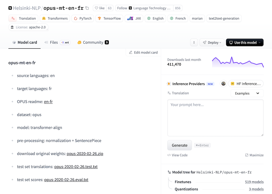
There are a range of Marian-compatible models on Hugging Face. As with the first post, we will focus on an OPUS MT English-to-French model known as Helsinki-NLP/opus-mt-en-fr. This is paired with inference implementation based on Hugging Face Transformers.
Hugging Face Transformers
The Hugging Face Transformers library supports models for text generation, machine translation, summarization and classification (just to name a few). It also provides support for training workflows, model configuration management, and interoperability with backends such as PyTorch and TensorFlow.
To streamline the experience of using a model, Hugging Face provides instructions for various Cloud AI providers and on your own system. Getting started with Helsinki-NLP/opus-mt-en-fr only requires a few lines of code:
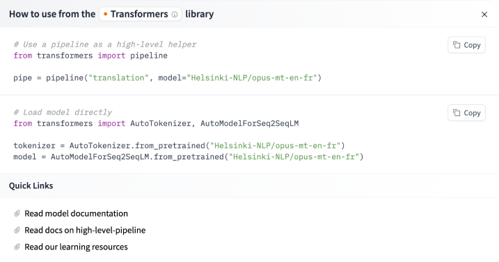
Hugging Face Transformers has a built-in Marian implementation, which makes getting started very easy!
MarianNMT vs MarianMT
The last thing to note is the difference between MarianNMT and MarianMT, which are easily confused…
When we say MarianNMT, we’re referring to the C++ toolkit introduced above. When we say MarianMT we’re referring to a Marian implementation based on Hugging Face Transformers. It comes with a set of pretrained models, and this is what we’ll use as the basis for our Rockchip NPU implementation.
Preflight
Let’s get MarianMT up and running, so that we have a baseline for the rest of this project. Note: Everything you see below should be executed on a PC.
The first thing we’ll need to do is install the transformers library, and some of its dependencies:
pip install \
  sentencepiece \
  torch \
  transformers
This command also installs compatible versions of PyTorch and SentencePiece, which are dependencies for MarianMT.
SentencePiece
You may have noticed on the Helsinki-NLP/opus-mt-en-fr model card earlier, that pre-processing includes “normalization + sentencepiece”. This means we’ll need to use Google’s SentencePiece library to tokenize input.
SentencePiece is an unsupervised text tokenizer and detokenizer, based on the byte-pair-encoding (BPE) and unigram algorithms. It is responsible for splitting a source text into subwords. We also use it to convert model output into human-readable sentences.
Test Script
We can put this all together using a simple Python script:
from transformers import MarianMTModel, MarianTokenizer
import torch

device = torch.device("cuda" if torch.cuda.is_available() else "cpu")
print(f"Using device: {device}")

model_name = 'Helsinki-NLP/opus-mt-en-fr'
tokenizer = MarianTokenizer.from_pretrained(model_name)
model = MarianMTModel.from_pretrained(model_name).to(device)

text = ["Hello, I am a fish. What kind of animal are you?"]

inputs = tokenizer(text, return_tensors="pt", padding=True).to(device)
translated = model.generate(**inputs)
translation = [tokenizer.decode(t, skip_special_tokens=True) for t in translated]

print(translation)
We’ve deviated from the model card a bit here, opting to use Marian-specific classes instead of relying on the AutoTokenizer and AutoModelForSeq2SeqLM. This is just for clarity.
The MarianTokenizer and MarianMTModel classes know how to tokenise input and transform, respectively. The tokeniser is also used to convert tokens generated by the model into human-readable output. MarianTokenizer does this using SentencePiece behind the scenes.
When we run the test script above, we see that it successfully translates the English phrase “Hello, I am a fish. What kind of animal are you?” into French:
$ python test.py
["Bonjour, je suis un poisson, quel genre d'animal êtes-vous ?"]
The marian-rknn repo contains a more robust version of this script, called preflight.py.
Note: The first time you run this script it will download the necessary pretrained model files. The model will be stored in a local cache, so that subsequent invocations don’t require another download.
PyTorch vs ONNX
The Hugging Face model downloaded above will be in PyTorch format, since that’s what Hugging Face Transformers uses internally. The question we need to answer is how to go from PyTorch format to RKNN format.
The key challenge is that RKNN Toolkit cannot just run or convert a PyTorch model by executing arbitrary Python code. We have two paths we can follow. The first uses TorchScript, which is a way to serialize and save models to disk so they can be used in alternative runtime environments (e.g. C++). Unfortunately, TorchScript has been deprecated since PyTorch 2.9.
Our second choice is ONNX - the Open Neural Network Exchange format. Once a model has been converted to ONNX, it is relatively easy to convert it to RKNN format. The ONNX runtime also supports the concept of Runtime Execution Providers, making it possible to run a model on a wide range of hardware platforms.
Converting to ONNX
With a little bit of research, we find that PyTorch directly handles ONNX exports. This seems relatively simple at first:
from transformers import MarianMTModel
import torch

model = MarianMTModel.from_pretrained('Helsinki-NLP/opus-mt-en-de')
dummy_input = torch.randint(0, 100, (1, 64))  # token IDs
torch.onnx.export(model, (dummy_input,), "marian.onnx", opset_version=13)
This would work well if you wanted to run the model on a GPU. In practice there’s more work required to export the model in a way that will cleanly convert to RKNN format and run on the Rockchip NPU. Thankfully, Kevin Costa’s Marian-ONNX-Converter project will save us a great deal of time and effort!
Marian-ONNX-Converter
Marian-ONNX-Converter does a few things that will be helpful for us. It exports a MarianMT model into a split encoder/decoder ONNX layout, and preserves the extra artifacts that are required to invoke the model outside of MarianMT. It also provides an ONNX implementation which can run on the CPU, or on a GPU using CUDA.
Marian-ONNX-Converter also happens to support quantization, which is important in embedded environments. However we disable quantization when converting from PyTorch to ONNX, as this would introduce layers into the model that are not supported by the RKNN API. We perform quantization later, when converting from ONNX to RKNN format.
To convert the PyTorch model we’ll first need to find the cached model path, which was downloaded during ‘Preflight’:
export MODEL_PATH=$(python -c "from huggingface_hub import snapshot_download; print(snapshot_download('Helsinki-NLP/opus-mt-en-fr'))")
We can then convert a model from PyTorch to ONNX:
python Marian-ONNX-Converter/convert.py $MODEL_PATH --no-quantize
We have to explicitly choose no quantization at this step, otherwise Marian-ONNX-Converter will attempt to quantize the encoder and decoder models in ways that are not supported by RKNN. It would also be premature to quantize the model before establishing baseline performance metrics. This will be the topic of part 3.
Note: I’m currently maintaining a fork of Marian-ONNX-Converter, which includes various small fixes that make it more appropriate for this project. This can be found here.
Model Files
Once we’ve converted the model to ONNX format, the output can be found in a sub-directory under outs/. In my case this was called outs/dd7f6540a7a48a7f4db59e5c0b9c42c8eea67f18, which was derived from the original model ID.
The contents of that directory should look something like this:
% ls -gho
total 1070376
-rw-r--r--  1    1.5K 13 Feb 21:59 config.json
-rw-r--r--  1    214M 13 Feb 21:59 decoder.onnx
-rw-r--r--  1    190M 13 Feb 21:59 encoder.onnx
-rw-r--r--  1    234K 13 Feb 21:59 lm_bias.bin
-rw-r--r--  1    116M 13 Feb 21:59 lm_weight.bin
-rw-r--r--  1    760K 13 Feb 21:59 source.spm
-rw-r--r--  1     74B 13 Feb 21:59 special_tokens_map.json
-rw-r--r--  1    784K 13 Feb 21:59 target.spm
-rw-r--r--  1    816B 13 Feb 21:59 tokenizer_config.json
-rw-r--r--  1    1.4M 13 Feb 21:59 vocab.json
As you might have guessed, the decoder.onnx and encoder.onnx files are ONNX models. These contain the model graphs and weights for the decoder and encoder, respectively. This is where attention happens!
The lm_weight.bin and lm_bias.bin files contain the weights and biases for the LM head. The raw output of a transformer is generally not in a form that is ready for human consumption. The LM head is a feed-forward neural network that converts transformer output into tokens that have meaning for humans.
The source.spm and target.spm files contain SentencePiece models for tokenization, and the vocab.json file ensures that tokens that occur in both the source and target languages are used efficiently. All other files in this directory are configuration files.
Converting to RKNN
Conversion from ONNX to RKNN format is relatively straight-forward, thanks to the RKNN Toolkit. We can simply load an ONNX model, then export that same model to RKNN format using the rknn.api module:
from rknn.api import RKNN

rknn = RKNN()
rknn.load_onnx(model='model.onnx')
rknn.build(do_quantization=False)
rknn.export_rknn('model.rknn')
We also want to convert the LM weights and biases from PyTorch format to raw floating point values:
def convert_weights(input_path, output_path):
    """Convert Torch LM head tensors to raw float32 for runtime matmul + bias.

    These can be loaded back into tensors in Python, or natively in C++.
    """
    tensor = torch.load(input_path, weights_only=True)
    weights = tensor.detach().numpy().astype(np.float32)
    weights.tofile(output_path)
    return weights
This is not strictly necessary, because our Python code can load the original lm_bias.bin and lm_weight.bin files directly, using PyTorch. However when we port the inference engine to C++, we will need raw floating point values. By converting now, we can be sure that our implementations behave consistently.
This conversion is handled by the rknn_convert.py script in my marian-rknn repo.
Quantization
In the example above, we’ve set do_quantization=False, which converts the model graph directly to RKNN format, with no quantization.
Quantization for encoder/decoder architectures is somewhat involved. For the encoder, we need to build a dataset containing a pair of NumPy files (the input IDs and attention mask) for each example. We then write the file names to a text file, one example per line.
Here’s what a dataset text file might look like:
calibration/input_ids_1.npy calibration/attention_mask_1.npy
calibration/input_ids_2.npy calibration/attention_mask_2.npy
calibration/input_ids_3.npy calibration/attention_mask_3.npy
calibration/input_ids_4.npy calibration/attention_mask_4.npy
calibration/input_ids_5.npy calibration/attention_mask_5.npy
...
The path to this file is then used as an argument for rknn.build():
rknn.build(do_quantization=True, dataset=calibration_path)
Effective quantization requires careful profiling and evaluation of a model, to ensure that performance does not suffer unnecessarily. I mention this mostly for completeness - We will leave quantization disabled for now, and instead cover this in detail in part three of this series!
Dynamic Ops
The next challenge we have is dynamic inputs. The Rockchip NPU has limited support for dynamic graph operations, which are required to handle inputs of arbitrary length. To avoid off-loading inference onto the CPU, we need to alter the model to use static input shapes.
For MarianMT we define these as:
ENCODER_INPUTS = ['input_ids', 'attention_mask']
ENCODER_INPUT_SIZE_LIST = [[1, 32], [1, 32]]

DECODER_INPUTS = ['input_ids', 'attention_mask', 'encoder_hidden_states']
DECODER_INPUT_SIZE_LIST = [[1, 32], [1, 32], [1, 32, 512]]
The array [1, 32] specifies an input length of 32 tokens for input_ids and attention_mask. The array [1, 32, 512] specifies an internal state with a shape of 32x512. The value 512 is not arbitrary - it is the size of the embedding used, which corresponds to d_model in the model’s config.json file.
The constants above are used when exporting the encoder and decoder models:
# Load encoder model
rknn = RKNN()
rknn.config(target_platform=platform,
            dynamic_input=[ENCODER_INPUT_SIZE_LIST])
rknn.load_onnx(model=encoder_path,
               inputs=ENCODER_INPUTS,
               input_size_list=ENCODER_INPUT_SIZE_LIST)

# Export encoder (trimmed for brevity)
rknn.build(...)
rknn.export_rknn(...)
rknn.release()

# Load decoder model
rknn = RKNN()
rknn.config(target_platform=platform,
            dynamic_input=[DECODER_INPUT_SIZE_LIST])
rknn.load_onnx(model=decoder_path,
               inputs=DECODER_INPUTS,
               input_size_list=DECODER_INPUT_SIZE_LIST)

# Export decoder (trimmed for brevity)
rknn.build(...)
rknn.export_rknn(...)
rknn.release()
Inference Engine
To keep things simple, our inference engine will be written in Python. Although there are potential benefits to writing an inference engine in C++, starting with Python has three main advantages:
- It will be faster to iterate. We do not need to worry about memory management, linking, and other C++ footguns.
- Interactions with SentencePiece will be closer to the original Hugging Face implementation, which will be helpful for comparison.
- Finally, we can take advantage of simulation mode in the RKNN Toolkit, to run the model on your development machine. This is much faster than transferring .rknn files to device for testing.
This section will be divided into five steps, introducing code snippets for each part of the translation process:
- Initialisation
- Tokenization
- Encoder
- Decoder Loop
- Detokenization
Let’s dive in!
Initialisation
During initialisation, we have to load each of the components of the model. This begins with two SentencePiece tokenisation models - one for the source language, and another for the target language:
# source language
spm_src = spm.SentencePieceProcessor(model_file=f"{input_path}/source.spm")

# target language
spm_tgt = spm.SentencePieceProcessor(model_file=f"{input_path}/target.spm")
We also need to load a vocab file, which maps token substrings to integers:
# load vocab from json file
vocab, vocab_inv = load_vocab(f"{input_path}/vocab.json", vocab_size)
Finally, we need to load the encoder and decoder RKNN models using RKNNLite:
# load encoder
rknn_enc = RKNNLite()
rknn_enc.load_rknn(f"{args.model_path}/encoder.rknn")

# load decoder
rknn_dec = RKNNLite()
rknn_dec.load_rknn(f"{args.model_path}/decoder.rknn")
Tokenization
You may wonder why we need two tokenizers and a vocabulary file. Surely a tokeniser would be sufficient for converting an input string into a series of integer token IDs…
There is a good reason for this. Marian allows the source and target languages to use the same token ID space. Say you have a token that appears in both the source and target languages (e.g. th), it can be more efficient to train the model using the same token ID for both languages.
The problem is that the two SentencePiece models are trained independently, leading common tokens to have different token IDs. The purpose of the vocab file is to correct this, by mapping token substrings to a common token ID space. This is best illustrated with a code snippet:
# break input string into token substrings
pieces = spm_src.encode(line, out_type=str)

# map token substrings to token IDs
tokens = [vocab.get(piece, unk_token_id) for piece in pieces]
These token IDs can then be used as input to the encoder.
Encoder
The encoder begins by building a fixed-length input_ids tensor. This is padded or truncated to the appropriate input length. The “end of stream” and “pad” tokens are part of the model configuration. We also need to build an attention_mask, in which valid token positions are marked as 1 and padded positions as 0. This gives the model visibility into which positions are meaningful and which are merely padding.
# prepare encoder inputs and attention mask
encoder_input_ids = prepare_encoder_inputs(tokens, enc_len, pad_token_id, eos_token_id)
attention_mask = build_attention_mask(encoder_input_ids, eos_token_id)
To invoke the encoder, we call rknn_enc.inference(...) with both arrays in the order expected by the model:
# invoke the encoder
encoder_outputs = rknn_enc.inference(inputs=[encoder_input_ids, attention_mask])
encoder_hidden_states = encoder_outputs[0]
The return value is a tensor (named encoder_hidden_states) which contains an embedded representation of each source token position. This will be used by the decoder to extract meaning from the source text.
Decoder Loop
Unlike the encoder, which runs just once, the decoder runs in an autoregressive loop. This means that each token generated depends on the output from previous iterations of the decoder.
The decoder requires three input tensors:
- Decoder input IDs (not the same as the input IDs passed to the encoder)
- The same attention mask prepared earlier
- The
encoder_hidden_statesproduced by the encoder
The first input is essentially the decoder’s “working memory”. On each iteration of the decoder, the model may attend to tokens that were previously generated. This helps inform which token is chosen next.
The third input is simply the output of the encoder.
We have a choice of two different decoding strategies, which are discussed further below:
if beam_search is None:
    # simpler, but input may be of slightly lower quality
    output_tokens = greedy_decode(
        rknn_dec,
        attention_mask,
        encoder_hidden_states,
        ...
    )
else:
    # more complex, but better output quality
    beam_width, beam_depth = beam_search
    output_tokens = beam_search_decode(
        rknn_dec,
        attention_mask,
        encoder_hidden_states,
        ...
    )
Greedy decoding is simpler, so we’ll focus on that for now. This snippet of code shows the entire decoder loop for greedy decoding:
def greedy_decode(
    rknn_dec,
    attention_mask,
    encoder_hidden_states,
    weight,
    bias,
    decoder_start_token_id,
    pad_token_id,
    eos_token_id,
    dec_len
):
    # prepare autoregressive decoder input; start by fully padding the tensor
    decoder_input_ids = np.full((1, dec_len), pad_token_id, dtype=np.int32)
    decoder_input_ids[0, 0] = decoder_start_token_id

    # this will hold our final decoder output
    output_tokens = []

    # main loop
    for step in range(dec_len - 1):
        # invoke decoder, passing in the three inputs
        outputs = rknn_dec.inference(inputs=[decoder_input_ids, attention_mask, encoder_hidden_states])

        # apply LM head, which converts the output into logits
        decoder_output = outputs[0]
        hidden = decoder_output[0, step, :].astype(np.float32)
        logits = hidden @ weight.T + bias

        # greedily decode next token by choosing the candidate
        # with the highest logit
        next_token = int(np.argmax(logits))
        output_tokens.append(next_token)

        # check for end of output
        if next_token == eos_token_id:
            break

        # otherwise, append token to decoder input for next iteration
        if step + 1 < dec_len:
            decoder_input_ids[0, step + 1] = next_token

    return output_tokens
The output of the decoder is a sequence of token IDs. The final step is to turn those token IDs into human-readable text!
Detokenization
Detokenization begins by inverting the vocab mapping applied earlier - converting token IDs into substrings. Those substrings are passed to the target tokenizer to be converted into human-readable text:
decoded_pieces = []
for token_id in output_tokens:
    if token_id in (eos_token_id, pad_token_id) or token_id <= 0:
        break
    piece = vocab_inv.get(token_id)
    if piece is not None:
        decoded_pieces.append(piece)

return spm_tgt.decode(decoded_pieces)
Decoding Strategies
In the decoder loop section above, we mentioned having two decoding strategies to choose from. These are Greedy Decoding and Beam Search. This choice is all about trade-offs.
Greedy decoding is fast and deterministic, picking the highest probability token at each step. Beam search explores multiple hypotheses in parallel, which often improves fluency or adequacy. However it also increases compute, memory pressure, and book-keeping costs.
Greedy Decoding
As tokens are generated, greedy decoding uses np.argmax(logits) to choose the highest probability token to append to the output.
An interesting observation we can make here is that logits are not the same as probabilities. Normally, we would use a Softmax function to convert the logits to probabilities:
# calculate softmax
logits -= np.max(logits)
exp_logits = np.exp(logits)
probs = exp_logits / np.sum(exp_logits)
In the case of greedy decoding, we can rely on the fact that argmax(logits) will identify the same token as argmax(probs).
Although efficient, the downside of greedy search is that the decoder cannot backtrack on tokens that lead to poorer translations.
Beam Search
Beam search addresses this by managing multiple candidate sequences at each step. The number of concurrent sequences (or beams) is known as the beam width.
To decide which beams should be extended, and which should be culled, the algorithm maintains a cumulative probability. After expanding each candidate beam with possible next tokens, only the top-ranked hypotheses are preserved.

Image Credit: Chapter 10.8 - Beam Search from Dive Into Deep Learning.
This diagram shows a beam size of 2 and maximum sequence length of 3. Greedy search can be treated as a special case of Beam Search where the beam size is set to 1.
Beam search reduces the risk of early mistakes dominating the final output. But it comes at the cost of compute, memory pressure and additional book-keeping. This extra work is primarily in the decoder and LM-head, which must be executed once per beam on each iteration.
Benchmarks
The final step in this process is benchmarking. How many sentences can the RK3588 translate per minute? Or more precisely, how many tokens?
Sample Text
To prepare for the benchmark, we need a file containing input sentences that are representative of what our system will encounter under real world conditions. The Random English Sentences dataset from Kaggle is a good place to start! Here’s what the first 10 lines look like:
I didn't know what to wear to my best friend's funeral.
There used to be a big cherry tree behind my house.
Sometimes, books and movies made her feel things she couldn't explain.
My bandaid wasn't sticky anymore so it fell off on the way to school.
He only had one drink but he's completely wasted.
In Hong Kong, everyone lives stacked together.
Her parents had been separated for almost three years, but she never expected them to actually go through with the divorce.
These are the things that I want from a relationship.
When one considers the issue from a different perspective, the answer seems to change.
She twisted her ankle and couldn't go to soccer anymore.
Benchmark Script
The marian-rknn repo includes a benchmark script (benchmark.py) which repeatedly translates input for a fixed period of time. Once complete, it prints throughput and token count statistics.
To run the benchmark, we have to provide a model path, a dataset, and a maximum runtime (in seconds). The benchmark will iterate over the dataset until the time budget is reached, then report aggregate throughput and per-stage timings:
python scripts/benchmark.py \
  outs/dd7f6540a7a48a7f4db59e5c0b9c42c8eea67f18 \
  datasets/en-phrases.txt \
  120 > results-greedy.txt
We can run the same test using Beam Search:
python scripts/benchmark.py \
  --beam-search \
  --beam-width 3 \
  outs/dd7f6540a7a48a7f4db59e5c0b9c42c8eea67f18 \
  datasets/en-phrases.txt \
  120 > results-beam-search.txt
Results
Here are the results!
As a baseline, greedy decoding with the datasets/en-phrases.txt dataset allowed us to produce 2766 output tokens. In total, we processed 207 sentences @ 1.705 sentences per second:
Benchmark complete
Elapsed: 121.442 s
Sentences: 207
Sentences/sec: 1.705
Total time: 121295.378 ms
Encoder time: 2492.285 ms
Decoder time: 91355.883 ms
LM head time: 26394.237 ms
Avg total time per sentence: 585.968 ms
Avg encoder time per sentence: 12.040 ms
Avg decoder time per sentence: 441.333 ms
Avg LM head time per sentence: 127.508 ms
Input tokens: 2379
Output tokens: 2766
Decoder iterations: 2766
Input tokens/sec: 19.590
Output tokens/sec: 22.776
When we run the same test with beam search enabled, and a beam width of 3, we see how much of an impact it can have…
Benchmark complete
Elapsed: 121.982 s
Sentences: 52
Sentences/sec: 0.426
Total time: 121851.846 ms
Encoder time: 631.315 ms
Decoder time: 72169.512 ms
LM head time: 20800.915 ms
Avg total time per sentence: 2343.305 ms
Avg encoder time per sentence: 12.141 ms
Avg decoder time per sentence: 1387.875 ms
Avg LM head time per sentence: 400.018 ms
Input tokens: 663
Output tokens: 729
Decoder iterations: 2177
Input tokens/sec: 5.435
Output tokens/sec: 5.976
Average decoder time per sentence goes up considerably, and the number of output tokens produced drops from 2766 to 729. Overall, we processed 52 sentences @ 0.426 sentences per second.
It’s worth noting that this is without any attempt at further optimisation.
Next Steps
Now that the model conversion and inference pipeline is working, we’re free to think about optimisation such as quantization. The promise of quantization is that we can reduce the memory footprint of model weights and activations, while also reducing compute overhead. But we need to be careful not to harm the overall performance of the model.
In part three, we will tackle quantization head on, looking at how to quantize a model, as well as how to evaluate the performance impact of doing so.
References
- Understanding SentencePiece
- Using dynamic input shapes on RKNN/RK3588 by Martin Chang
- Marian-ONNX by Kevin Costa
- Unlocking On-Device AI by John OSullivan
- RKNN API Demo by Rockchip
- Quantize ONNX Models