Machine Translation at the Edge: Part 1
This is my third post exploring Edge AI, with a focus on the Rockchip RK3588 NPU. This post dives into Machine Translation, a Natural Language Processing task that has traditionally been associated with Cloud AI services. With advances in Edge AI hardware, model architectures and distillation techniques, it is now feasible to perform Neural Machine Translation directly on an embedded device.
The goal of this post (and the next) is to build a Neural Machine Translation pipeline for the Rockchip NPU. We’ll walk through model selection, quantization, and deployment using the RKNN Toolkit. Python and C++ source code will be available on GitHub. The initial implementation is based on the Khadas Edge2 development board, but should be easy to port to other RKNN-based devices.
If you haven’t already, I recommend reading the first and second posts, as they cover helpful background material.
Contents
- Machine Translation
- RKNN Platform
- RKNN Model Zoo
- MarianNMT vs MarianMT
- Test Flight
- Next Steps
- References
Machine Translation
Machine Translation is a technique used to automatically, or mechanically, translate text (or speech) from one language to another. We generally refer to the two languages involved as the ‘source’ and ‘target’ languages. At a high level, the machine reads text in the source language, and generates a corresponding translation in the target language.
Machine Translation has been an active area of research since the early 1950s. In fact, one of the first conferences on Mechanical Translation (as it was known at the time) was hosted at MIT in 1952. With such a rich history, there are many translation models to choose from. We’ll briefly review some earlier architectures here.
Statistical Models
Human language is highly redundant. After seeing the first few letters of a word we can often predict the following letters with fairly high accuracy. The same is true for words in a sentence, and even phrases. This motivates the treatment of language as probabilistic in nature.
In Statistical Machine Translation (SMT), a model learns a probabilistic mapping from a source language to a target language. A classic example of this is Phrase-Based Machine Translation (PBMT). A sentence is first segmented into phrases, and each phrase is mapped to corresponding phrases in the target language:
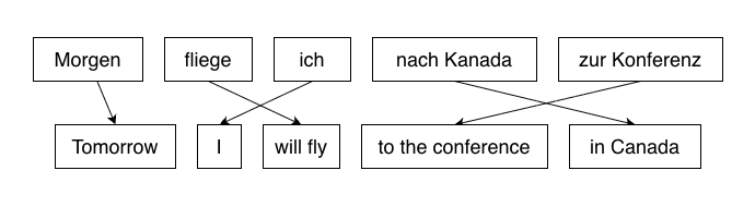
Image credit: Adapted from the original image found here.
This was included in the ACL 2005 Workshop on
Building and Using Parallel Texts.
Once candidate word/phrase matches have been selected, the system searches for the best overall translation by ranking and re-ordering the translations, before combining them to produce a fluent result.
Aside: Moses
If you start digging into the literature around statistical models, you are likely to stumble upon Moses, an open-source SMT system. Although Moses is no longer common in front-line translation systems, it is still relevant for ‘low-resource’ language research (i.e. translating languages with limited training data) and as a teaching tool.
You may also discover Sacremoses, a Python port of Moses’ text preprocessing scripts. This is often used in older model pipelines, or as an optional dependency. SentencePiece, BPE and Unigram tokenizers are more common these days.
The primary issue with SMT systems is that they depend on a pipeline of hand-crafted components. Because translation occurs across multiple stages (e.g. segmentation, alignment, phrase tables, and reordering) errors in early stages can easily propagate to the final translation. The result ends up being brittle and expensive to maintain.
Encoder-Decoder Models
Encoder-Decoder models replace the individual components of SMT and PBMT with a single end-to-end model that can learn directly from a large collection of source-target language pairs. This works remarkably well on high-resource languages (i.e. those with plenty of high-quality training data).
Another reason that Encoder-Decoder architectures have been so successful is that Machine Translation is fundamentally a sequence-to-sequence problem - you take a variable-length source sentence and produce a target sentence. The source and target sentences will often be different lengths, since an expression in one language may look very different in another.
Even within the sub-category of Encoder-Decoder models, we have a few variations to consider… the first are Recurrent Neural Networks.
RNNs and LSTMs
Recurrent Neural Networks (RNNs) are designed for processing sequential data, where the order of elements is important. This is clearly the case for language, where the meaning of a word depends on the presence and order of words (or more generally, tokens) around it.
Unlike feed-forward networks (FFNs), which process inputs independently, RNNs utilize recurrent connections. These recurrent connections carry ‘hidden state’ from one iteration to the next - allowing the network to progressively capture the meaning in a sentence. This is well suited to translation, where the source sentence is first processed by an Encoder RNN to extract the meaning, then passed to a Decoder RNN to generate output tokens:
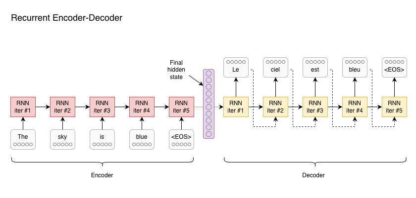
Some information is passed on from each iteration of an RNN to the next - this is the hidden state of the RNN. In this architecture, the source sentence is processed by the encoder RNN, until the final token is seen (<EOS>, or ‘End of Sequence’). The final hidden state is then used to initialise the decoder RNN, which generates tokens until <EOS>.
RNNs do suffer from some limitations, such as inherently sequential execution, and difficulty with long-range dependencies. They also have a fixed-sized hidden state vector, which limits representational capacity. Since an entire sentence must be squeezed into a fixed-size vector, RNN-based models may struggle with longer sentences.
Transformers
The most recent Machine Translation models tend to use some variation of the Transformer Architecture, which we covered in the previous post on Tiny Language Models.
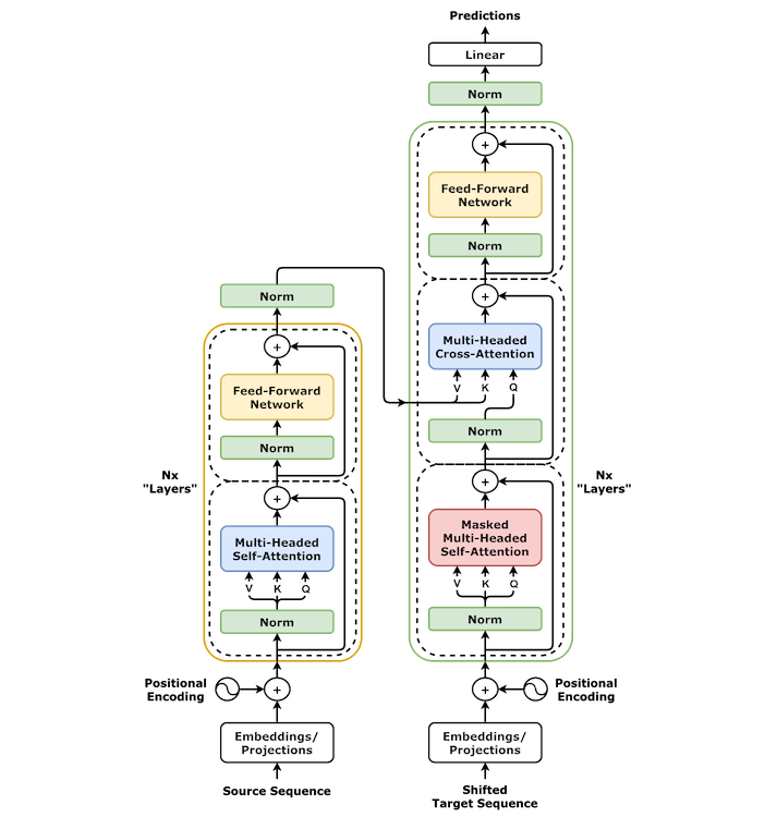
Image Credit: Wikipedia.
Unlike RNNs, Transformers do not rely on recurrent hidden state. They instead use Self-attention, which allows each token to incorporate information from all other tokens in the sequence. This is implemented in such a way that all tokens can be processed in parallel, which addresses one of the major bottlenecks of RNNs.
After the encoder has processed a sentence, the decoder typically generates one token at a time, conditioned on the previously generated tokens.
Together, these characteristics make the Transformer architecture particularly well suited to Machine Translation, and this is the kind of architecture we’ll be discussing throughout the rest of this exercise.
RKNN Platform
Let’s move on to our target platform - this includes our choice of our hardware and framework support.
Why use the Edge2?
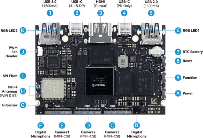
The target for this exercise is the Khadas Edge2. This compact hobbyist board is based on the Rockchip RK3588 SoC, an 8-core 64-bit ARM processor with a dedicated neural processing unit (or NPU).
The RK3588 SoC uses a Unified Memory Architecture (UMA). In practice, this means the CPU and NPU operate on memory that is allocated from the same pool of system memory. This is different to discrete desktop GPUs, where the CPU and GPU each have their own pool of memory and often results in large data transfers over PCIe.
Platform Limitations
While UMA simplifies communication between the CPU and NPU, we need to be mindful of allocation constraints (e.g. contiguous blocks of memory, required for DMA) and monitor overall memory pressure. Large models can easily lead to out-of-memory errors and allocation failures.
Bandwidth is also shared, so concurrent CPU and NPU workloads compete for DRAM throughput even if memory capacity is sufficient. Our preference is to find smaller models that are specialised to the task at hand, rather than more generalised large language models.
RKNN Toolkit
To take advantage of hardware acceleration on the Rockchip NPU, we need to interface with the RKNPU driver via the RKNN API. Rockchip’s RKNN Toolkit is an SDK for the Rockchip NPU that supports model conversion in Python (on PC), and inference/evaluation on Rockchip devices.
The toolkit supports conversion, quantization and fine-tuning models on PC. It also includes runtime and C/C++ headers that we need to interface with the NPU in C++:
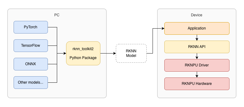
The RKNN Toolkit includes components that run on-device (for inference), and others that are intended to be run on a PC (for model construction and conversion).
A typical RKNN workflow begins with a pretrained model in PyTorch, TensorFlow or ONNX format. RKNN Toolkit includes Python APIs to load models from other formats, and export them in RKNN format:
from rknn.api import RKNN

rknn = RKNN()
rknn.load_onnx(model='model.onnx')
rknn.build(do_quantization=True, dataset='dataset.txt')
rknn.export_rknn('model.rknn')
Once in RKNN format, a model can be loaded on-device using C++ or Python code.
Model Support
Although there are RKNN implementations for some popular model architectures, most pretrained models will be published in other formats. Common formats in the wild include PyTorch and TensorFlow. Another common format is ONNX, short for Open Neural Network Exchange. This has gained popularity as a model interchange format.
The RKNN API makes it easy to load and export models, but whether this will be sufficient depends heavily on the model architecture. In some cases, it may be impossible to run a model on the Rockchip NPU due to certain layers or operations not being supported. For example, models that rely on dynamic graph operations are not well supported.
When converting models, it can be helpful to visualise the model graph, in order to diagnose problems. Netron is a convenient and easy-to-use viewer for neural networks:
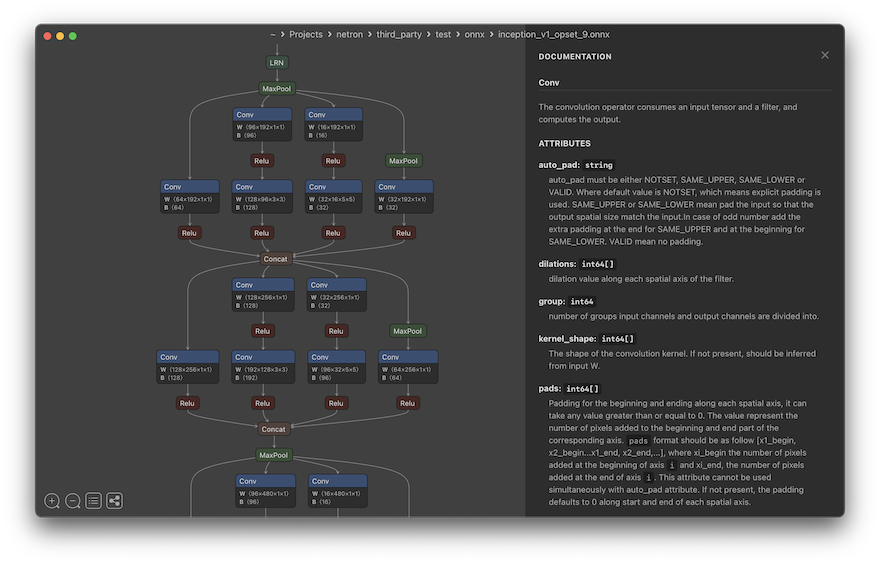
Image credit: Screenshot taken from the Netron GitHub repo.
RKNN Model Zoo
When implementing a machine learning model, it is generally a bad idea to start from scratch. Let’s look at some of the available examples.
The RKNN Model Zoo provides a range of examples for the Rockchip platform, primarily computer vision models. But there is one we can use for Machine Translation, based on a model architecture known as the Lite Transformer.
Lite Transformer
The Lite Transformer is a variant of the Transformer model that makes certain trade-offs to improve performance on resource constrained devices. The authors recognised that computation in a standard Transformer is dominated by the feed-forward network (FFN). This is despite the fact that the FFN comes after Attention, and so does not mix context across tokens.
A straightforward way to reduce compute demands is to shrink the embedding size directly - this reduces capacity across the entire model. Alternatively, we can reduce the attention feature dimension. While bottlenecking attention can save compute, the FFN still dominates compute, and the savings can be limited relative to the quality hit.
The authors introduce a clever solution to this problem, called Long-Short Range Attention.
Long-Short Range Attention
Long-Short Range Attention (LSRA) splits the representation into two parallel branches - a convolutional neural network, specialised for learning short-range dependencies between tokens, and an attention block that can focus on long-range dependencies.
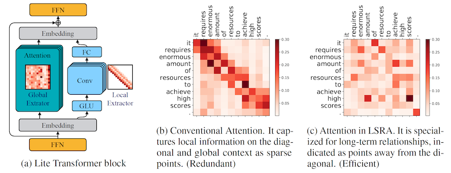
Image Credit: Figure 3 from Lite Transformer with Long-Short Range Attention by Wu et al. This shows how conventional attention predominantly captures local (short-range) dependencies (b). In LSRA, the presence of the convolutional network for local context allows the attention mechanism to better capture long-range dependencies (c).
The Lite Transformer authors use a threshold of 500M multiply-add operations to measure performance of the model in a mobile setting. By configuring various models to operate within this threshold, they showed that LSRA often outperforms pure transformer models in resource-constrained environments.
Other Choices
While models such as Lite Transformer have great potential for reducing computational cost on embedded devices, there are some trade-offs we need to consider. The two we’re most concerned about are availability of pretrained models, and additional challenges in fine-tuning.
For this post, I’ve shortlisted several alternatives that directly address the needs for model availability and fine-tuning:
-
Google’s T5 is a versatile text-to-text transformer, capable of a variety of NLP tasks, including translation and summarization. T5 uses a generalised model that needs to be prefixed with the specific task (e.g.
"Translate English to French: I am a fish."). Possibly too big for our embedded use-case, especially if we only need to support one language pair. -
MarianNMT is a pure C++ toolkit specialised for training Neural Machine Translation (NMT) models. It is often faster in inference, and capable of producing higher quality models for specific language pairs. Marian has been used in production systems by Microsoft and Mozilla (via their own fork). Strong contender!
-
OpenNMT is similar to MarianNMT in that it provides an ecosystem for NMT and neural sequence learning. The OpenNMT project also maintains CTranslate2, an efficient inference engine for transformer models. Also a strong contender!
While CTranslate2 includes support for AArch64 (ARM 64-bit) CPUs, our ideal target is the Rockchip NPU. Both OpenNMT and MarianNMT will require a custom inference implementation and model conversion process. Due to the availability of model checkpoints for Marian, that’s where we’ll focus our attention going forward.
MarianNMT vs MarianMT
As mentioned above, MarianNMT is a toolkit specialised for training NMT models. Somewhat confusingly MarianMT (without the N) refers to a collection of Transformer-based encoder–decoder models, published on Hugging Face.
All MarianMT variants follow the Transformer architecture, with 6 layers in both encoder and decoder. They are all natively ONNX exportable, which is good for us, because it eases the transition to RKNN format.
For training, MarianMT relies on the MarianNMT framework, which is written in C++. Marian can run on the CPU, however GPU acceleration is available via CUDA/cuDNN when enabled.
The MarianNMT project includes an efficient inference engine, also written in C++. This can be compiled to run on the CPU, or on an NVIDIA GPU using CUDA. We can also use an implementation based on Hugging Face Transformers.
Build from Source (Optional)
Getting started with MarianNMT is relatively straightforward… assuming you have a Linux system with an NVIDIA GPU, and the necessary CUDA Toolkit / cuDNN libraries installed.
To begin with, you can clone the MarianNMT source code from GitHub:
git clone https://github.com/marian-nmt/marian.git
cd marian
Then we can build it using CMake:
mkdir build && cd build
cmake ..
make
This builds the entire toolkit, which includes tools for training and the inference engine.
The MarianNMT build depends on CUDA by default, so you won’t have much luck if you try to build this on macOS or another platform without CUDA support. To try compiling without CUDA support:
cmake .. -DUSE_SENTENCEPIECE=on -DCOMPILE_CPU=on -DCOMPILE_CUDA=off
make
This will be somewhat slower, but good enough for a simple test run.
Note: This may not work on newer Macs based on Apple Silicon. Don’t worry if this means you cannot run the examples yourself. I’ve included example output below, so you can follow along!
NPZ Format
Unfortunately, Hugging Face checkpoints aren’t directly usable by the Marian C++ decoder. The MarianNMT inference engine expects an .npz file…
The Marian .npz format is essentially a ZIP archive containing one or more .npy (NumPy) arrays, which store model weights in a format appropriate for Marian NMT models. It is based on NumPy’s .npz format and is specifically tailored for fast loading and execution in the C++ Marian decoder.
We can see how this works with a simple Python script:
import numpy as np

# Save arrays to an npz file
a = np.array([1, 2, 3])
b = np.array([4, 5, 6])
np.savez('arrays.npz', array1=a, array2=b)

# Load arrays from an npz file
data = np.load('arrays.npz')
print(data['array1'])  # Output: [1 2 3]
print(data['array2'])  # Output: [4 5 6]
One way we can address this is to convert a pretrained model from another format (e.g. PyTorch) to .npz format. However, this can be error-prone, and it’s an unpleasant way to begin experimenting with a new architecture.
Pretrained Models
Alternatively, we can find pretrained models that already have .npz files available. There are a range of models available, trained on various language pairs and datasets. Common datasets for Machine Translation include:
- WMT - WMT (short for ‘Workshop on Machine Translation’) is a shared-task dataset created annually for Workshop on Machine Translation competitions. Includes major language pairs and is trained on news, formal text, and curated sources.
- Tatoeba - A community driven dataset consisting of example sentences and translations, all provided by volunteers. This includes hundreds of languages, including many ‘low resource’ languages.
- OPUS - OPUS (Open Parallel Corpus) is an umbrella project hosting hundreds of parallel corpora from many domains, scraped from the web or public sources. Great for translation, as it contains billions of sentence pairs across 400+ languages.
Test Flight
For the rest of this post, we’ll focus on an English <-> French model that was pretrained on the OPUS dataset.
Getting the Model
The specific model we want is en-fr from the OPUS-MT-train repo on GitHub. The model is a few years old now, having been trained in 2020. However, it’s in NPZ format, ensuring that we can use it directly with MarianNMT.
The model’s README file provides a link to a download mirror. Let’s download and extract the model:
wget https://object.pouta.csc.fi/OPUS-MT-models/en-fr/opus-2020-02-26.zip
unzip -d opus-2020-02-26 opus-2020-02-26.zip
Note: The instructions below assume you’ve extracted the model to marian/build/opus-2020-02-26.
The zip file will be about ~265MB, and the extracted model will take about 288MB on disk. The file list when extracting may be a bit intimidating at first:
Archive:  opus-2020-02-26.zip
  inflating: opus-2020-02-26/README.md
  inflating: opus-2020-02-26/LICENSE
  inflating: opus-2020-02-26/opus.spm32k-spm32k.transformer-align.model1.npz.best-perplexity.npz
  inflating: opus-2020-02-26/opus.spm32k-spm32k.vocab.yml
  inflating: opus-2020-02-26/opus.spm32k-spm32k.transformer-align.valid1.log
  inflating: opus-2020-02-26/opus.spm32k-spm32k.transformer-align.train1.log
  inflating: opus-2020-02-26/source.spm
 extracting: opus-2020-02-26/source.tcmodel
  inflating: opus-2020-02-26/target.spm
  inflating: opus-2020-02-26/decoder.yml
  inflating: opus-2020-02-26/preprocess.sh
  inflating: opus-2020-02-26/postprocess.sh
There are several files that are worth pointing out. The first is opus.spm32k-spm32k.transformer-align.model1.npz.best-perplexity.npz, which contains Marian model weights in NPZ format. This is the core of the model. The string spm32k tells us that the specific tokenizer is SentencePiece (spm) with a vocab size of 32,000.
The next two files of interest are source.spm and target.spm, which are SentencePiece models. These models contain the information needed to segment an input sentence into tokens (i.e subword parts), and to concatenate generated tokens into the final output. This leads us to a more in-depth discussion on tokenization…
Tokenization
When translating a piece of text, that input must first be segmented into units of text called tokens. Tokens may be entire words, individual characters, or groups of characters (i.e. subwords):
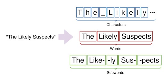
Token granularity is an implementation detail that must be included in a model definition. MarianNMT often uses SentencePiece to tokenize text into subwords. SentencePiece itself supports the Unigram and Byte-Pair Encoding (BPE) algorithms. Which one is used is model-dependent.
To make this more concrete, we can use Marian’s spm_encode to tokenize an input sentence ("I am a spiky fish") using the source tokenizer:
$ echo "I am a spiky fish" | ./spm_encode --model opus-2020-02-26/source.spm
I ▁am ▁a ▁sp ik y ▁fish
We can see that the output is a series of tokens (or subword parts), but our model requires integer token IDs. The last file we’re interested in is opus.spm32k-spm32k.vocab.yml - this provides a ‘vocabulary’, mapping tokens to integers (and vice-versa).
Vocab File
The vocab YAML file is human readable, so we can take a peek inside… This is the first 20 lines of opus.spm32k-spm32k.vocab.yml:
$ head -n 20 opus-2020-02-26/opus.spm32k-spm32k.vocab.yml
</s>: 0
<unk>: 1
",": 2
.: 3
▁the: 4
▁de: 5
"'": 6
▁of: 7
▁la: 8
s: 9
▁and: 10
▁et: 11
▁to: 12
▁des: 13
▁l: 14
▁a: 15
▁les: 16
▁à: 17
▁in: 18
▁le: 19
The list begins with </s> and <unk>, which represent end-of-sequence and unknown strings, respectively. Unknown strings occur when the input contains character sequences that do not have a valid mapping.
Next, we see some common symbols , and ., followed by strings that look like parts of words. These are often prefixed with a whitespace marker ▁, which bears a striking resemblence to an underscore… The whitespace marker means that these are prefixes - the first part of a word that occurs after a space. This distinction between subwords that follow a space and those that don’t has been shown to improve model performance.
Full Pipeline
With all that covered, we can invoke the model using a Unix pipeline consisting of three executables: spm_encode, marian-decoder and spm_decode.
We can invoke the decoder using this rather complicated command:
echo "I am a fish" \
  | ./spm_encode \
      --model opus-2020-02-26/source.spm \
  | ./marian-decoder \
      --models \
        opus-2020-02-26/opus.spm32k-spm32k.transformer-align.model1.npz.best-perplexity.npz \
      --vocabs \
        opus-2020-02-26/opus.spm32k-spm32k.vocab.yml \
        opus-2020-02-26/opus.spm32k-spm32k.vocab.yml \
      --devices 0 \
      --beam-size 6 \
      --normalize 1.0 \
  | ./spm_decode \
      --model opus-2020-02-26/target.spm
Starting at the top, we use echo to output the string "I am a fish". This is piped to spm_encode so that SentencePiece can tokenize the input. Tokens are then piped to marian-decoder.
Note that when we invoke marian-decoder, the same vocab file is provided twice - this is not a typo. Marian models support asymmetric translation - i.e. using different vocabularies for the source language (encoder) and target languages (decoder). Therefore, the marian-decoder command expects paths for both source and target vocabulary files. As we saw above, this file contains a mix of English and French tokens, so we can use the same file for both.
Finally, the output of marian-decoder is piped to spm_decode to be converted into human-readable text!
[2026-01-04 19:53:04] [config] Loaded model has been created with Marian v1.8.2 2111c28 2019-10-16 08:36:48 -0700
...
[2026-01-04 19:53:05] Loaded model config
[2026-01-04 19:53:05] Loading scorer of type transformer as feature F0
[2026-01-04 19:53:05] [memory] Reserving 284 MB, device gpu0
[2026-01-04 19:53:05] [gpu] 16-bit TensorCores enabled for float32 matrix operations
[2026-01-04 19:53:05] Best translation 0 : ▁Je ▁suis ▁un ▁poisson
Je suis un poisson
[2026-01-04 19:53:05] Total time: 0.05016s wall
If we comb through the output, we find the string ‘Je suis un poisson’, which is a valid French translation of ‘I am a fish’!
Next Steps
That completes our introduction to machine translation and the MarianNMT toolkit. We’ve covered a lot of ground! However, everything we’ve done so far has been on PC, rather than our target device.
In part two, we turn our attention to the Rockchip NPU. Our goal will be to perform MarianMT inference on the Rockchip NPU. We will download a pretrained MarianMT model from Hugging Face, convert it to RKNN format, then run it directly on Rockchip NPU.
To make all of this work, we’ll need to consider quantization, input padding and layer compatibility. Thankfully, the RKNN Python API makes this much easier than it sounds. Our result will be a Marian implementation that runs directly on the Rockchip NPU!
References
Historical:
- MIT Conference on Mechanical Translation - Mostly unpublished papers from the early days of Machine Translation.
- Moses SMT - This is worth exploring, if only to appreciate the extensive research that went into constructing Machine Translation systems prior to the rise of Transformers.
NMT Systems:
Tokenization:
- Byte-Pair Encoding - Hugging Face
- Unigram - Hugging Face
- Understanding SentencePiece - A nice introduction to SentencePiece.