Tiny Language Models
This post continues on the theme of Edge AI. We previously covered the basics of Edge AI and the practicalities of running YOLO, an Object Detection algorithm, on the Rockchip NPU. In this post, we’ll look at the history and scaling challenges of Large Language Models and what it means to train and deploy a tiny language model.
Although there is an example for the Khadas Edge2 at the end, the content here is mostly foundational in nature. In a later post, we will look at practical examples of running Machine Translation algorithms on the Rockchip NPU.
Contents
- A Brief History of Language Models…
- Large Language Models
- Transformer Architecture
- Tiny Language Models
- Tokenization
- RKLLM Toolkit
- Next Steps…
- References
A Brief History of Language Models…
The history of language models (or more generally, Natural Language Processing) features some clearly visible paradigm shifts. In the early days of computing, computer scientists and programmers were quick to explore the AI landscape. As early as the 1960s, chatbots such as of Joseph Weizenbaum’s ELIZA led people to believe that the era of machine intelligence was upon us.
Fast forward to the 1980s and 90s, and by this time N-gram models had taken hold. These probabilistic models aimed to predict words and symbols that would occur in a text, using the surrounding context to condition the probability. Although the results were compelling, they had properties that made them very difficult to scale.
In the early 2000s, neural networks were successfully applied to language modeling. The immense representational power of neural networks enabled the development of word embeddings, like those seen in Word2Vec. Although vanilla neural networks quickly reached their limits, research in the 2010s gave us Recurrent Neural Networks and LSTMs, which allowed neurons to preserve state from one word/symbol to the next.
Finally, the invention of Transformers in 2017 ushered in the era of Large Language Models. You can see from the timeline below that we’re currently in a period of rapid growth, marked not just by leaps in computational capacity, but also paradigm shifts:
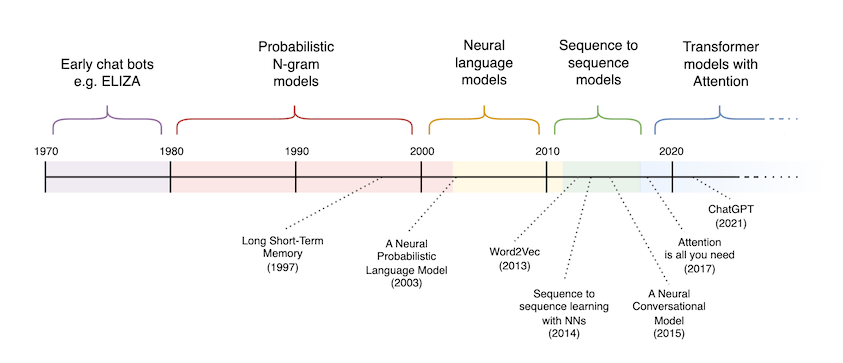
We’ll dive into each of these in a bit more detail.
N-gram Models
N-gram models are purely probabilistic language models, trained on a body of text (commonly known in NLP as a “corpus”) to capture the frequency and context in which different symbols occur. Symbols can be individual characters, words, or even sub-words (e.g. prefixes and suffixes).
N-gram models are characterised by the length N of the input sequence used to condition the probability of a symbol that follows in the sequence. Assuming that entire words are used as symbols:

Using Bayes’ rule (or Bayes’ theorem), we can calculate the probability of a given input sequence as a joint probability:
\[\begin{aligned} &P(\text{The}\text{ }{sky}\text{ }{is}\text{ }{blue}) \\ = &P({The}, {sky}, {is}, {blue}) \\ = &P({The}) * P({sky}\text{ }|\text{ }{The}) * P({is}\text{ }|\text{ }{The}, {sky}) * P({blue}\text{ }|\text{ }{The}, {sky}, {is}) \end{aligned}\]N-gram models suffer from two critical limitations. First—they have limited expressive capabilities. Specifically, the probability of a particular symbol occurring may be dependent on context that falls outside the conditioning sequence. We can attempt to address this by increasing N to capture more context.
This leads to the second issue - as the value of N increases, the data and storage requirements also grow exponentially. And if the dataset is not sufficiently large and diverse, the model risks overfitting.
Neural Language Models
The introduction of Neural Language Models in 2003 also gave us the concept of Word Embeddings. A Word Embedding is a vector representation of a word, where each component in the vector corresponds to some concept captured by the model.
Let’s make this more concrete. Say you have a vocabulary of five words, and each word is represented using its one-hot encoding:
Cat    -> [1, 0, 0, 0, 0]
Kitten -> [0, 1, 0, 0, 0]
Dog    -> [0, 0, 1, 0, 0]
Puppy  -> [0, 0, 0, 1, 0]
Bird   -> [0, 0, 0, 0, 1]
If we used these vectors as inputs for a neural network, the input layer will require five neurons: one for each component of the input vector. Unfortunately, as the vocab grows in size, say to 40,000 words, the input layer of our neural network will also grow to be 40,000 neurons wide.
Besides scaling issues, one-hot encoding comes with two other disadvantages:
- Sparsity - Most values in each vector are zeros. This is wasteful of storage, and means that the first layer of the network has relatively little information to work with.
- No Relationships Between Words - The disjoint nature of one-hot vectors means that we cannot derive any meaningful relationships between words.
To highlight the second point, consider the first two examples: Cat and Kitten. A Kitten is a kind of Cat, so it doesn’t make sense for those to be completely disjoint in their representations. Word Embeddings address this by learning a dense representation (an embedding) for each word in the dataset. The embedding reduces the dimensionality of the input data, allowing the rest of the model to operate on vectors with a lower dimensionality.
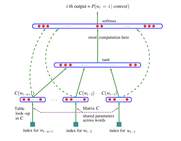
Image Credit: Figure 1 from A Neural Probabilistic Language Model by Bengio et al (2003).
The major contribution of Bengio et al’s paper was train a neural language model end-to-end.
Word2Vec
A critical issue with Neural Language Models is that training at scale was expensive and suffered from tight coupling between network architecture and word representations. In 2013, Word2Vec showed that it was possible to learn meaningful relationships between words by training a shallow network on a large corpus. The resulting word embeddings could then be re-used across different architectures.
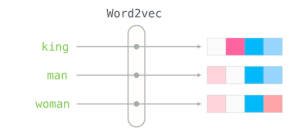
Image Credit: The Illustrated Word2Vec by Jay Alammar.
He goes into great detail about how Word2Vec can be used in a variety of applications.
Recurrent Neural Networks
Recurrent Neural Networks (RNNs) made it possible to preserve some state from one token to the next. This meant that generated tokens would take more context into account - for example, choosing the generated token based on the meaning implied by the most recent words in the input sequence.

Image Credit: A Brief Overview of Recurrent Neural Networks from Analytics Vidhya.
A key problem with RNNs is vanishing gradients. Long Short-Term Memory (LSTM) networks build upon RNNs by introducing a new internal structure…
Long-Short Term Memory Networks
Although the idea for Long Short-Term Memory (LSTM) networks was first described in 1997 by Hochreiter et al, it wasn’t until the 2010s that this found wider adoption in Language Models. LSTMs attempt to solve the vanishing gradient problem by ensuring that errors flow back through the network, while introducing gating mechanisms that allow the error (or gradient) to be truncated when it is beneficial.
However, this wasn’t quite enough to get us to where we are now… RNNs and LSTMs are inherently serial, which causes severe bottlenecks. Vanishing gradients are a problem, even in LSTM networks. This makes it increasingly difficult for models to learn connections between tokens over longer time spans.
Transformers
The NLP landscape changed dramatically in 2017, when the seminal paper Attention Is All You Need introduced the Transformer architecture. The Transformer architecture replaces recurrence with a mechanism called “Attention.” This made it possible for language models to capture long-range dependencies.
You’re almost certainly aware of Transformers (although you may not recognise them by name). They are the “T” in GPT (short for Generative Pre-trained Transformers) and have led to many state-of-the-art results in Natural Language Processing and Machine Learning tasks.
Large Language Models
Current state of the art language models contain billions of parameters, and must be trained on massive datasets. As a reference point, we’ll use OpenAI’s GPT-3, since there are some reasonably well grounded numbers available online.
Just the pretraining phase of GPT-3 relied on approximately 570GB of text content, pulled from sources such as Common Crawl, OpenWebText2 and Wikipedia. Prior to training, this content is converted to tokens through a process called tokenization. The resulting training set contains approximately 300 billion tokens.
The largest GPT-3 model uses 175 billion parameters. This translates to roughly 350GB if you store the weights as 16-bit floating points (FP16). This poses many architectural challenges, even when working with data-center class GPUs. It is currently impossible to load so much data onto a single GPU. Therefore, the weights for Large Language Models must be distributed across multi-GPU clusters, with the clusters themselves connected via high-bandwidth interconnects.
Hardware Constraints
So what do we do when we want to run a Large Language Model on an embedded device?
We face a number of challenges when targeting an embedded environment. First is limited memory (RAM/VRAM). LLMs use a lot of RAM for model weights and context windows. Besides limited RAM, the memory architecture may not be as fast as desktop / server RAM.
Next is limited computing power. While many embedded devices now feature NPUs (Neural Processing Units) these are still very limited compared to desktop and server-grade GPUs.
Model Architecture Support
Finally, model architecture support may be limited. Embedded NPUs are simpler in nature than desktop and cloud GPUs. They often lack some of the hardware-accelerated operations required to implement a model using the Transformer architecture. Those operations need to be implemented using slower CPU-based emulation.
Attention kernels and rotary embeddings are two examples that are often not supported.
Transformer Architecture
Understanding the Transformer Architecture will get us a little closer to the question of why language models are so large in the first place. We’ll briefly touch upon the concepts of Self-Attention, Cross-Attention, and the model structures typically seen in LLMs.
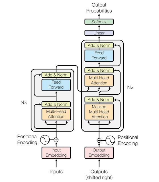
Image Credit: Figure 1 from Attention Is All You Need.
Self-Attention
Self-Attention is a mechanism that allows each token in a sequence to decide which other tokens are relevant to it and to aggregate that information via a weighted sum. The result is a context-dependent token representation, which can “look” backwards as well as forwards in the input sequence.
This is in contrast to RNNs and LSTMs—these models could pass context forward from one state to the next; however, they were restricted to encoding that information in hidden state that was of a fixed size. They also suffered from vanishing gradients, and were unidirectional in nature.
Scaled Dot-Product Attention
We hand-waved an important detail above: the weighted sum.
Each token’s initial representation is projected into query, key, and value vectors. The query vector is used to calculate a similarity score with the keys for every other token in the sequence. We then apply a softmax to the similarity scores to find attention weights. Those weights are used to calculate a weighted sum of the corresponding value vectors. The final result is a context-dependent representation of a token. This whole process is called Scaled Dot-Product Attention.
\[\text{Attention}(Q, K, V) = \text{softmax}\left( \frac{Q K^\top}{\sqrt{d_k}} \right) V\]That paragraph was a lot to digest! If this is new to you, I highly recommend the Neural Networks course from 3blue1brown. Specifically, the content on Attention in Transformers.
Cross-Attention
Scaled Dot-Product Attention is also used in Cross-Attention. Where Self-Attention asks “How do tokens in this sequence relate to one other?”, Cross-Attention asks “How do tokens in this sequence relate to tokens in another sequence?”
Both Self-Attention and Cross-Attention use the Scaled Dot-Product Attention formula that we saw above. The only difference is how we construct Q, K, and V.
In Self-Attention, Q, K, and V are all derived from the same sequence of hidden states. You can think of this as trying to predict the next token in a single sequence.
In Cross-Attention, Q comes from one sequence, while K and V come from another, distinct sequence. So you can think of this as trying to predict the next token in an output sequence, given the tokens seen in a different input sequence.
Encoders and Decoders
Cross-Attention was originally developed to support Machine Translation and Text Summarisation tasks. In these architectures, one half of the model is known as the Decoder, and the other half is the Encoder. Cross-Attention allows the decoder to attend to outputs of the encoder, while generating a distinct sequence of tokens. This allows the output to reflect the meaning of the original input, but transformed in some meaningful way - e.g. translated to a different output language.
The basic structure of an Encoder-Decoder Architecture is shown below:
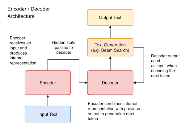
It’s also possible to have encoder-only or decoder-only models. Google’s BERT is an example of an encoder-only model, while GPT is an example of a decoder-only model. In both cases, only Self-Attention is used.
The key difference between GPT (decoder-only) and BERT (encoder-only) lies in how they are trained. BERT is trained using a bidirectional approach, whereby tokens are permitted to attend to any other token in the input text. GPT is unidirectional, and uses masking techniques to ensure that the model cannot “look into the future”.
Model Structure
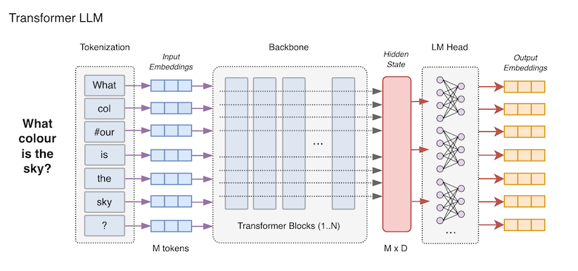
Transformer models tend to follow a similar architecture.
The first part of the model is the tokenizer—this is the part of the network that splits the input into individual tokens. We explore this in more detail in the Tokenization section below.
Following the tokenizer is the backbone. This is the core of the neural network, implementing the attention mechanism used by the model to generate an output sequence. However, the output of this layer cannot be used as-is. It’s a highly specialised representation of the model’s hidden state.
The last part of the model is the head (sometimes called the “LM head”). This is a standard linear layer that projects each hidden state to a vector of size vocab_size. This vector is used to choose tokens (essentially the reverse of tokenisation), based on the confidence assigned to each possible token.
Recommended Resources
We’ve skipped over many other details, such as Positional Encoding, which are important to understand when diving into LLMs. To learn more, I recommend picking up a copy of Hands-On Large Language Models by Jay Alammar and Maarten Grootendorst.
Hands-on Large Language Models covers a wide range of topics. Beyond just LLM fundamentals, it explores different ways to chain models together to build sophisticated LLM-powered applications.
Tiny Language Models
With Large Language Models out of the way, we can shift our attention to Tiny Language Models.
Tiny Language Models are typically trained using fewer parameters or other simplifications such that they will fit within the constraints of an embedded device. We’ll look at just a few here, but be aware there are many others!
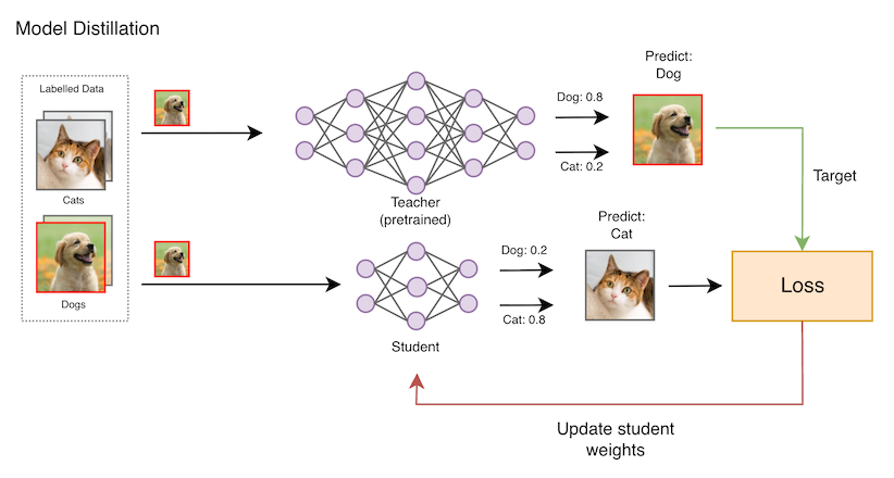
Model Distillation
A key ingredient in creating Tiny Language Models is model distillation. This is the process by which a compact “student” model can be trained using the outputs of a much larger “teacher” model. This allows the student model to capture concepts learned by the teacher, without direct exposure to the training set.
TinyLlama
TinyLlama is a compact language model that copies the architecture and tokenizer of Llama 2 (Meta’s open-source language model) but shrinks the parameter count to make it compatible with modest GPUs, CPUs, and edge devices. With just 1.1B parameters, TinyLLama is approximately 150x smaller than GPT-3.
Because TinyLlama is architecturally compatible with Llama 2, it can be used with many existing Llama-based tools and projects, and there are multiple downstream variants mirroring those of the base model. For example, the TinyLlama-1.1B-Chat variant is fine-tuned on the UltraChat dataset.
Qwen
Qwen (also known as Tongyi Qianwen) is a family of large language models developed by Alibaba Cloud. Qwen is released in a variety of model sizes (all published on Hugging Face), so it’s likely that you’ll find one that fits within your constraints.
At time of writing, the latest iteration is Qwen 3. However, earlier iterations are often preferred for embedded AI, due to their smaller size and simpler architectures. Another advantage of Qwen is that it is released with open weights and a permissive license, and it sits in a sweet spot for “tiny” and “mid-size” local models.
The underlying architecture also works well with quantization schemes. Quantization reduces the precision of model weights and activations, making it easier to fit within the constraints of an embedded device. We’ll look at a Qwen variant in the example at the end of this post.
TinyBERT and DistilBERT
TinyBERT and DistilBERT are both distilled versions of Google’s 2018 language model, BERT.
DistilBERT (released by Hugging Face in 2019) is basically a smaller BERT (66M parameters) that you can fine-tune like normal, with no custom distillation pipeline required. What this means is that you can fine-tune the smaller model directly. In practice, it may perform slightly worse than full BERT, but it can be good enough for many applications while offering better speed and reduced memory usage.
TinyBERT, from Huawei’s Noah’s Ark Lab, uses a two-stage distillation approach (first pass is general, then task-specific). It comes in 4-layer and 6-layer versions. The 4-layer variant is even smaller than DistilBERT (just 14.5M parameters) and considerably faster while offering similar accuracy. The 6-layer variants typically use 67M parameters, depending on configuration.
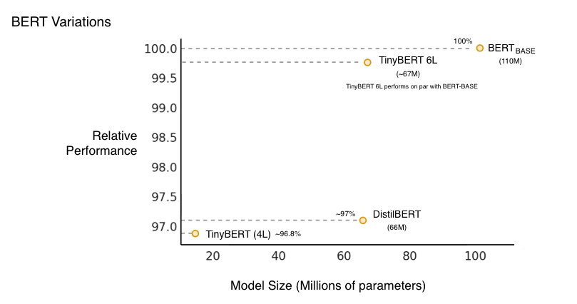
DistilBERT is often preferable unless you rely on the very small footprint offered by the TinyBERT 4-Layer variation. TinyBERT’s more aggressive distillation process may come at the cost of some accuracy. However, this may be a worthwhile trade-off when building for Edge AI devices.
Tokenization
Tokenization is the very first step in processing text input - it is the process by which raw text input is broken down into smaller units that can be handled by a language model. This critical first step reduces the length of the sequence that a model has to process, while retaining important context.
Tokenization is a deceptively broad topic, and although it’s a critical component in modern SOTA language models, we won’t cover it in great detail here. It really deserves its own post!
Kinds of Tokenization
There is, unfortunately, no one-size-fits-all approach to tokenization. First of all, we have determine whether we want tokens that represent characters, words, or sub-words:
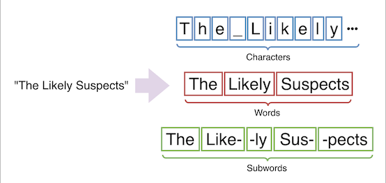
Some models even operate on entire sentences - in this case we would break a text into individual sentences, which are processed in their entirety. This is generally NOT relevant these days.
While sub-word tokenization is currently the most common approach used in SOTA models, character-based (or tokenization-free) models have begun to gain traction. We’ll skip of tokenization-free models here, and focus on Sub-Word Tokenization.
Sub-Word Tokenization
In Sub-Word Tokenization, we break text into smaller units that are larger than characters but smaller than full words.
Key algorithms are Byte-Pair Encoding (BPE), WordPiece and Unigram.
Byte-Pair Encoding
BPE starts with a vocabulary of individual characters and iteratively merges the most frequent pair of symbols until a desired vocabulary size is reached. Merges based on the frequency before adding to the vocabulary.
Let’s look at how BPE would be used to choose a set of tokens for the string AAABDAAABAC:
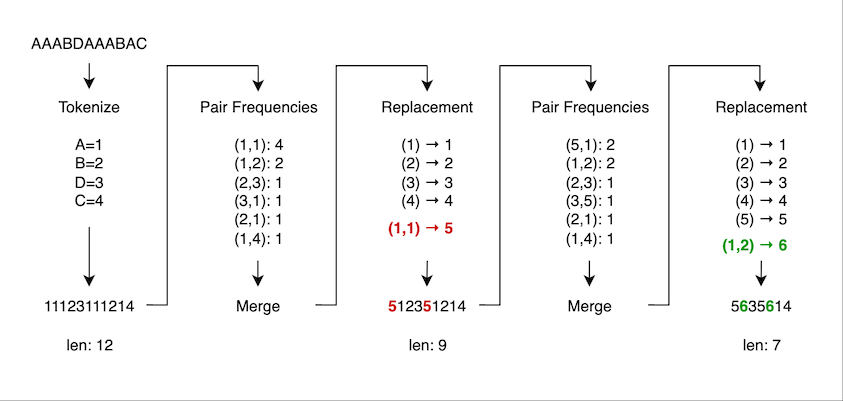
In the first step, we have just one token ID per character. We then calculate the frequency of each pair of adjacent tokens across the training set. The most frequent pair is merged, and given its own token ID. The training set is updated to use the new token. This process repeats until the desired number of tokens has been generated.
WordPiece
WordPiece is similar to BPE in that it iteratively merges subword units, starting from characters. However, instead of choosing the most frequent pair like BPE, WordPiece uses a probability-based score that approximates how much a new merged symbol would improve the likelihood on the training data.
Unigram
Unigram starts with a large vocabulary of potential sub-words and iteratively removes the least likely ones until the optimal set is found.
You may also see SentencePiece mentioned in the context of tokenization. SentencePiece is an unsupervised text tokenizer and de-tokenizer that implements Byte-Pair Encoding (BPE) and the Unigram language model.
De-Tokenization
The output of a language model often depends on the inverse of tokenization. The LM Head of the model is responsible for converting an internal representation of a sentence or document into a series of tokens, often using the same mapping as the original model input. Those tokens are then converted into human-readable text via de-tokenization.
De-tokenization may be a probabilistic process. If the language model outputs a confidence level for each possible token, then tokens may be sampled according to confidence assigned to them. This can have a huge impact on the quality of the output, and several different approaches are used.
Greedy Decoding
If we want the fastest output, and can tolerate some mistakes, then the simplest option is Greedy Decoding. We always choose the token with the highest confidence. However, these days Beam Search is more popular.
Beam Search
Beam Search aims to strike a balance between Greedy Decoding and an exhaustive search for the best possible output sequence. The idea is that we keep a certain number of partial solutions in memory, determined by the beam size K. At the first time step, we choose the K most probable tokens, based on the logits generated by the model.
On all subsequent steps, we extended each candidate sequence by one token, and re-evaluate the joint probability of that particular sequence occurring. All but the top-K sequences are discarded, and then the process continues. I highly recommend reading Chapter 10.8 - Beam Search from Dive Into Deep Learning to learn more about the inner workings of Beam Search.
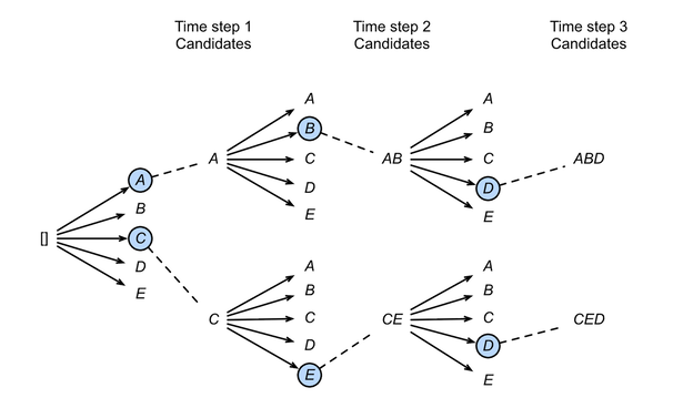
Image Credit: Chapter 10.8 - Beam Search from Dive Into Deep Learning.
This diagram shows a beam size of 2 and maximum sequence length of 3. Greedy search can be treated as a special case of Beam Search where the beam size is set to 1.
RKLLM Toolkit
RKLLM-Toolkit is a software development kit published by Rockchip, that supports model conversion and quantization on a desktop PC. It also includes a device runtime with C/C++ APIs for Rockchip NPUs, making it possible to deploy language models to Rockchip devices.
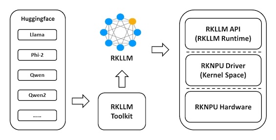
Image Credit: RKLLM-Toolkit repository on GitHub.
Getting started with RKLLM
Khadas makes it very easy to get started with LLM demos on the Edge2. While the documentation is a bit light, there isn’t actually that much to it.
Assuming you’re running a Linux distribution on your Edge device, you should find a script named khadas_llm.sh in your path. Running this will install dependencies, clone the rknn-llm repo and prompt you download/builds models.
CMake already installed, skipping installation
Repository exists, skipping clone

======================
System Memory: 15.5G
Available Models:
 1) DeepSeek 1.5B        [Missing]
 2) DeepSeek 7B          [Missing]
 3) Qwen2 2B-VL          [Missing]
 4) ChatGLM3 6B          [Missing]
======================
Download missing models? [y/N]
Unfortunately, the first time I tried this, the models failed to download due to 404 Not Found errors. I eventually found the correct files on dl.khadas.com:

From here, I simply modified the khadas_llm.sh script, making the following replacement:
dl.khadas.com/development -> dl.khadas.com/resources/development
                                           ^^^^^^^^^
After doing this, it was smooth sailing!
Available downloads:
 1) DeepSeek 1.5B
 2) DeepSeek 7B
 3) Qwen2 2B-VL
 4) ChatGLM3 6B
Select model to download: 1
Downloading DeepSeek 1.5B...
The model we want is 1) DeepSeek 1.5B. The full name for this model is DeepSeek-R1-Distill-Qwen-1.5B.
NOTE: the order may be different if you run this script on your own device.
DeepSeek-R1-Distill-Qwen
DeepSeek-R1-Distill-Qwen-* is a series of open-weight reasoning-focused language models where DeepSeek’s larger R1 reasoning model has been distilled into a Qwen 2.5–based backbones. This model is available in 1.5B, 7B, 14B, 32B parameter variations. We use the 1.5B parameter model in the example below.
When you first download the DeepSeek-R1-Distill-Qwen-1.5B model, it will be stored in a generic format such as ONNX. Certain conversion steps need to take place before running on the Rockchip NPU:
- Converting the model graph to use Rockchip-compatible operations
- Layer fusion, which is a kind of optimisation
- Quantization, to reduce the precision of model weights to fit within device constraints
This is called building the model. We covered these in my previous post on Edge AI.
The khadas_llm.sh script can do this for you automatically. Simply follow the prompts to build the model:
Building DeepSeek 1.5B model...
-- Configuring done (0.0s)
-- Generating done (0.0s)
-- Build files have been written to: /home/khadas/rknn-llm/examples/DeepSeek-R1-Distill-Qwen-1.5B_Demo/deploy/build/build_linux_aarch64_Release
[100%] Built target llm_demo
[100%] Built target llm_demo
Install the project...
-- Install configuration: "Release"
-- Up-to-date: /home/khadas/rknn-llm/examples/DeepSeek-R1-Distill-Qwen-1.5B_Demo/deploy/install/demo_Linux_aarch64/./llm_demo
-- Up-to-date: /home/khadas/rknn-llm/examples/DeepSeek-R1-Distill-Qwen-1.5B_Demo/deploy/install/demo_Linux_aarch64/lib/librkllmrt.so

Configure runtime parameters (press Enter for defaults)
Max new tokens (default 2048):
Example Prompt
Finally, we can enter some text to see how the model responds. Let’s try asking how many planets are in the solar system…
user: How many planets are there in the solar system?
robot: <think>
Okay, so I need to figure out how many planets there are in our solar system. Hmm, let me start
by recalling what I know about the solar system. I remember that it's a system of eight planets
orbiting the sun. But wait, isn't there something called Pluto as well? I think it was considered
a planet for a long time but later it was classified as a dwarf planet because its size is too
big and it doesn't have an atmosphere.

So, if there are eight planets in total, including Pluto, then excluding Pluto, how many would be
left? Let me count: Mercury, Venus, Earth, Mars, Jupiter, Saturn, Uranus, and Neptune. That's
eight. But wait, I think sometimes people include Pluto as a planet too, so maybe the count is
nine.

I should also consider if there are any other planets besides these eight. From what I know, our
solar system has eight planets: Mercury, Venus, Earth, Mars, Jupiter, Saturn, Uranus, and Neptune.
There aren't any others in our galaxy or beyond it that we can observe as planets right now. So,
excluding dwarf planets like Pluto, there are eight.

I wonder if there's a different way to count them. Maybe including some gas giants or something
else? No, I don't think so. Each planet is distinct and has its own orbit around the sun without
overlapping with others in terms of size or distance from it. So, each one is unique in their
characteristics.

Wait, could there be any other planets that are not considered planets by modern definitions?
I'm pretty sure all eight are recognized as planets now. There's also the asteroid belt and the
Kuiper Belt, but those aren't planets themselves; they're regions of space with many asteroids.

So, putting it all together, if we count each planet individually, there are eight in our solar
system. If we include Pluto, then it's nine. But since Pluto is no longer recognized as a planet,
I think the correct answer is eight.
</think>

There are 8 planets in our solar system. These are Mercury, Venus, Earth, Mars, Jupiter, Saturn,
Uranus, and Neptune. Pluto was once considered a planet but is now classified as a dwarf planet
due to its size and lack of atmosphere.

**Answer:** There are 8 planets in the solar system.

--------------------------------------------------------------------------------------
 Stage         Total Time (ms)  Tokens    Time per Token (ms)      Tokens per Second
--------------------------------------------------------------------------------------
 Prefill       318.77           14        22.77                    43.92
 Generate      33152.13         482       69.91                    14.30
--------------------------------------------------------------------------------------
Next Steps…
Machine Translation
This content in this post started as just one section of a deep-dive into Machine Translation at the Edge, which looks at implementing a machine translation system on the RK3588 NPU. Keep an eye out for that post!
Tokenization Deep Dive
While writing this, I also found myself writing at length about different tokenisation methods, and the latest developments in token-free language models. That content has also been moved to a separate draft, and I hope to have both posts published by the end of the year.
References
As usual, I drew upon dozens of resources while preparing this post. The list below contains a selection of links that I think will be useful to someone wanting to dive deeper into the topics covered in this post. They’re listed roughly in the same order as the topics were covered.
Word Embeddings
Attention
GPT
- Language Models are Unsupervised Multitask Learners - This is the paper that introduced GPT-2
- Language Models are Few-Shot Learners - This is the paper that introduced GPT-3
Tokenization
- Hugging Face - Unigram Tokenization
- Mastering Tokenization in NLP: The Ultimate Guide to Unigram and Beyond!
- Let’s build the GPT Tokenizer - Andrei Karpathy’s talk on BPE
Text Generation
