Edge AI using the Rockchip NPU
Ever wondered what it takes to run real-time object detection and face recognition on a tiny device, without the cloud? I’ve been exploring this recently, while testing the limits of the Khadas Edge2. Powered by a Rockchip RK3588 processor - with a built in neural processing unit - this little Edge AI device packs quite a punch. And it’s all neatly packaged for consumers and hobbyists alike.
This post is split into three parts. Part 1 will begin with a brief tour of the Edge AI problem space, the kinds of AI models that are available, and technical details of the Edge2. In Part 2, we’ll dive into the software and example code available for Rockchip devices, and explore some popular computer vision datasets. Finally, Part 3 will make this more practical, walking through the steps to train a custom object detector.
Contents
- Part 1: Edge AI
- Khadas Edge2
- Low Level Details
- Applications
- Part 2: Software and Datasets
- Khadas Resources
- Quantization
- Datasets
- Part 3: Transfer Learning
- YOLOv5
- Building a Dataset
- Training the Model
- Closing Thoughts
Part 1: Edge AI
Let’s start from the top.
You may already be familiar with Cloud AI, thanks to services such as ChatGPT, or even Google Search, with its introduction of AI generated content into search results. If Cloud AI is one end of the AI spectrum, this post focuses on the other end of that spectrum - machine learning algorithms running on local hardware devices. This is generally refered to as Edge AI, or AI at the Edge. Naturally, there is an appropriately named O’Reilly book on the topic:
To learn more about the book, visit the O’Reilly website.
Some commonplace examples of Edge AI devices include modern mobile phones, smart appliances, and cars with self-driving or driver-assist features. These are cases where a reliable internet connection may not be available, or safety concerns require that AI processing happens with low latency.
Example Applications
Edge AI isn’t limited to the examples above. You’ll also find AI in the following embedded settings:
- Smart Cameras: Detecting intruders or anomalies without needing to stream footage to the cloud.
- Voice Control: Processing voice commands locally (e.g., wake word detection).
- Manufacturing: Identifying defects on the production line.
- Retail: Monitoring customer foot traffic and shelf inventory in real time.
- Healthcare: Tracking bio-signals locally for faster diagnosis.
With all these examples, it’s not difficult to find some common themes as to why Edge AI can be desireable:
- Being able to react to data or signals in real-time, without needing to send data to the cloud. Lower latency means faster, more responsive UX.
- Offline operation, independent of an internet connection. This means Edge AI works even when you’re on a flight, or stuck in a tunnel.
- Preservation of privacy. Personal data never leaves the device, which can be critical for privacy-focused users, or heavily regulated industries such as healthcare.
Constraints
A key challenge with Edge AI is that devices often have constrained compute, memory, and power budgets that inherently restrict model complexity. This is especially true in the Embedded Systems space. In the most extreme cases, Edge AI may need to run on microprocessor devices such as the Arduino. Of course, it’s common these days to use more powerful alternatives, such as the Arduino Portenta H7:
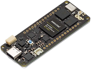
Image Credit: The Arduino store.
The Portenta H7 features an STM32H747 processor, with two cores - a Cortex-M7 and a Cortex-M4. The separation of these cores means that the device can handle real time control and AI processing simultaneously. However, this processor is not designed for compute-heavy AI tasks such as object detection and real-time video analysis.
Model Updates
The embedded nature of Edge AI devices also leads to difficulties in shipping model updates. Regulatory constraints may require that models are trained and rigorously tested up-front. And once a device is deployed, it may be costly (or even illegal) to update the model. Bandwidth and storage can also be an issue. Some state of the art (SOTA) models may be hundreds of megabytes in size (or even gigabytes), making distribution impractical.
Training vs Inference
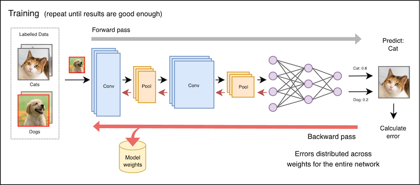
Implementation of a machine learning algorithm can be broken down into two key phases: Training and Inference.
During the training phase, a machine learning algorithm is exposed to a dataset from which it can extract (or ‘learn’) patterns and other meaningful relationships. The output of training are the parameters for a model, e.g. connection weights for a neural network. Training tends to be computationally expensive, and requires access to training data. On each pass through the dataset (known as an ‘epoch’), the network predicts the labels associated with each example in the dataset. Those predictions are compared with the true labels, and the error is distributed across the weights in the network:
In the inference phase, the parameters (or weights) learned in the training phase are loaded into memory, and used by the model to process previously unseen inputs. The weights are rarely altered at runtime.
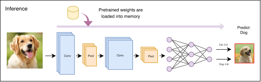
This storage cost for training data is prohibitive for Edge AI applications, and the data itself may be proprietary. As such, Edge AI applications typically focus on efficiency for inference, rather than training.
Khadas Edge2
This takes us to the Khadas Edge2.
The Edge2 is a slim and compact ARM PC that is designed with Pogo Pads, FPC headers and MIPI-Interfaces which makes it convenient for developers to access the necessary I/O for embedded applications. It includes HDMI output, two USB-A ports, and two USB-C ports, for data and power:
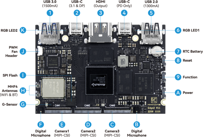
The MIPI ports on the bottom edge of the board allow three cameras to be connected directly to the device, for advanced video processing tasks.
Rockchip RK3588
The chip that powers all of this is the Rockchip RK3588S2, an 8-core 64-bit ARM processor. This includes a dedicated NPU (neural processing unit), making it possible to run deep learning inference on-device, without needing a GPU or access to a Cloud AI service. This makes the RK3588 ideal for real world Edge AI applications such as surveillance, robotics, or smart sensors.
The Rockchip NPU has direct access to system memory, and supports INT8, INT16 and FP16 precision models natively. We’ll discuss the importance of precision further in the Numeric Precision section below.
Power Consumption
A critical characteristic of embedded devices is power consumption (along with it’s first cousin, heat dissipation). Embedded devices are often battery-powered, or deployed in locations where it is difficult to provide active cooling.
The Edge2 balances strong performance with very modest power consumption. While under load, Thermal Design Power (TDP) is estimated to be between 5-10W. This is especially appealing when compared to using a desktop GPU, which can easily have a TDP 30-50x greater. The NPU can handle up to 6 TOPS (Trillions of Operations Per Second) - very impressive given the power budget.
Khadas’ documentation recommends a 24W power supply, which will provide ample headroom for powering connected peripherals.
Community Support
On the software side, Rockchip supports several options for deploying models to the device - these include RKNN Toolkit, ONNX, and LiteRT (“Lite Runtime”, formerly known as TensorFlow Lite). RKNN Toolkit provides tooling for converting various model formats into RKNN Format, which run natively on the RK3588 NPU.
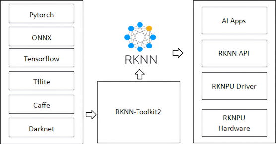
Image credit: RKNN Toolkit documentation.
This means you can build and train models in popular frameworks (e.g. PyTorch or TensorFlow) before converting them to run natively on the Rockchip NPU. Rockchip maintains an extensive RKNN Model Zoo on GitHub, which includes example code for many popular models.
Finally, Khadas provides extensive documentation for working with the Edge2 itself, and growing community interest around Rockchip devices on Reddit - see the r/RockchipNPU subreddit.
Compared to NVIDIA Jetson
Many developers are discovering that these RK3588 boards compare very favourably against NVIDIA Jetson or Raspberry Pi for Edge AI inference. The Khadas Edge2 offers competitive edge AI performance at a lower price point than NVIDIA Jetson Xavier NX or Orin.
Multiple I/O options, including M.2, USB-C, GPIO, and HDMI, make the Edge2 suitable for integrating into smart cameras, drones, or custom enclosures.
Low Level Details
Let’s dive deeper into the capabilities of the device, and how inference on an embedded device is different to other environments.
Floating Point
When talking about floating points numbers, or ‘floats’, we usually refer to decimal numbers that are represented using 32-bits. These bits can be broken down into three parts: a sign, an exponent, and a fraction (the ‘mantissa’). This is in accordance with the IEEE 754 standard, which describes how these bits can be interpreted as a decimal.
It’s beyond the scope of this post to explain how all this works. The most intuitive explanation I’ve seen for this is Fabien Sanglard’s Floating Point Visually Explained. And for much more detail, I recommend What Every Computer Scientist Should Know About Floating-Point Arithmetic.
Numeric Precision
The RK3588 SoC has a dedicated NPU that natively supports models with INT8, INT16 and FP16 numeric precision. These refer to 8-bit integer, 16-bit integer, and 16-bit floating point precision, respectively. These are pretty self-explanatory - INT8 is a signed integer, represented using 8 bits. This means it can take values between -128 and 127. Naturally, INT16 is 16 bits, covering a range between -32768 and 32767.
There are several numeric representations commonly used in Machine Learning:
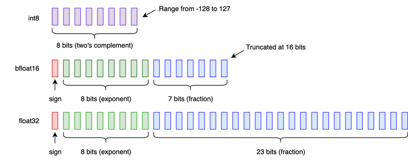
This determines the numerical precision of the weights and activations used during inference, but it is generally NOT the same as the precision used during training. What usually happens is that a model is trained at a higher level of precision (e.g. FP32 or 32-bit floating point) on a desktop or cloud GPU, before being converted for use on the target device.
Memory Architecture
This is another area where the Edge2 differs from a desktop GPU. The Edge2 comes with up to 16GB of LPDDR4 RAM, which is shared by the CPU, GPU, and NPU. This shared memory architecture means data can be easily shared between different processing units, without the overhead of transferring memory from one device to another.
By comparison, the RAM for an NVIDIA desktop GPU is independent of main system memory. While NVIDIA offers a ‘Unified Memory’ solution that allows system memory and GPU memory to share the same address space, this is simply a convenience for the programmer - it does not avoid the need to transfer data between physical devices.
Applications
Now that we know a bit about the kind of device we’re working with, what are some applications that are well suited to it?
Object Detection
Object Detection is a classic computer vision task that involves identifying, classifying and locating objects within an image or video feed. The key questions that object detection algorithms (attempt to) answer are:
- How many objects are present? (Identification)
- What kinds of object are they? (Classification)
- Where are they are located? (Localisation)
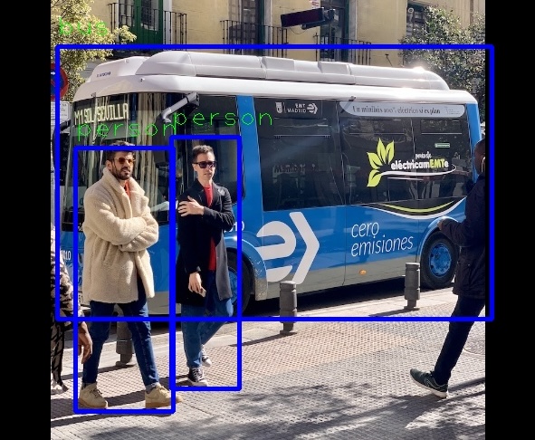
Image Credit: Output from Khadas example code for SSD Object Detection
Some common models for Object Detection include SSD (Single Shot Detector), RetinaNet, and Faster R-CNN. Another popular choice is YOLO (short for “You Only Look Once”), which we’ll examine in more detail in the second part of this post.
Facial Recognition
Facial Recognition is a classic computer vision problem, generally broken down into two distinct tasks:
The first is Face Detection, where we would like to locate all of the faces in an image, similar to how Object Detection is primarily concerned with locating objects.
The second is Face Recognition, which has a range of additional applications, such as providing biometric security for personal devices. As you would expect, there are many models available. Just to list a few:
-
FaceNet (Google, 2015) - This model introduced the concept of face embeddings using triplet loss. The model is trained using example ‘triplets’, each consisting of three separate face images. FaceNet provides a good performance baseline, however newer models may offer superior embedded performance.
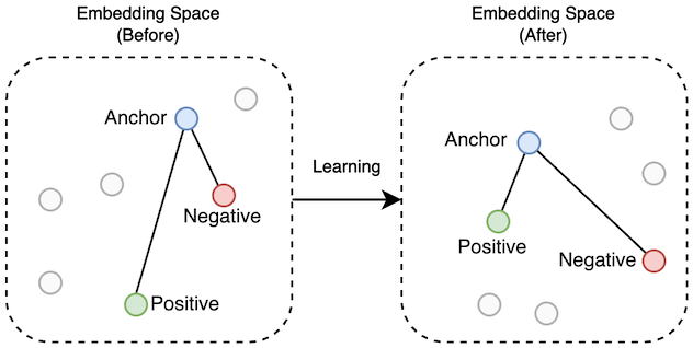
Triplet Learning: Positive examples move closer to the anchor, negative examples move further away.
-
RetinaFace - RetinaFace builds upon the RetinaNet object detection model, adding the ability to detect human faces and predict key facial landmarks (eyes, nose, corners of the mouth).
See the original paper RetinaFace: Single-stage Dense Face Localisation in the Wild for more detail.
-
ArcFace or MagFace - ArcFace and MagFace are two newer state-of-the-art models for Face Recognition.
ArcFace (2018) introduces a variation of the Softmax Loss function (often referred to referred to as Cross Entropy Loss), which encourages same-class samples to have embeddings closer to one another, while different-class samples are further apart. What this means in practice is tighter clustering of the same person’s face, and clearer separation between different faces.
MagFace (2021) builds on ArcFace by incorporating the magnitude of each embedding to the quality of the input face image. Higher-quality face images yield larger embedding magintudes. This allows MagFace to not only maintain strong recognition performance but also provide a built-in measure of face quality, which can be valuable in real-world applications.
Sentiment Analysis
Sentiment Analysis typically refers to the identification of tone, attitude or emotion present in text or speech. For example, in an e-commerce setting, we could classify online reviews as positive, neutral or negative. For audio or speech, Sentiment Analysis can be used to detect emotional states (e.g. delight, stress or frustration).
When analysing recordings of speech, sentiment can be inferred from acoustic features. These include:
- Pitch
- Loudness
- Tone of voice
- Pauses and rhythm of speech
These may be derived from a Mel Spectrogram:
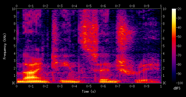
Image Credit: Spectrogram of the spoken words “nineteenth century” from Wikipedia.
A Mel Spectrogram has the frequency axis converted to the mel scale, which is designed to match human auditory perception.
Analysis of text tends to be more subtle, as it may not capture emotional nuances. This can be improved by adding more context. Alternatively, more samples may be required to accurately determine the tone of a body of text.
Part 2: Software and Datasets
Now that we have the lay of the land, let’s see what tools are available for the Edge2 specifically, starting with libraries and tooling from Rockchip.
RKNN Toolkit
RKNN-Toolkit2 is an SDK from Rockchip that supports model conversion, inference and performance evaluation on PC and Rockchip NPU platforms. On the PC side, it supports model conversion and quantization workflows. On the device side, it facilitates loading and running models on the Rockchip NPU, using C/C++ or Python APIs.
The primary purpose of the toolkit is to take models that have been trained on PC, and convert them into a format that will work with the the RKNN API. Once a model has been concerted to RKNN format, we run inference on a Rockchip NPU using the RKNN C API or Python API. The toolkit contains several examples written in both C++ and Python.
It’s worth noting that RKNN models are sensitive to input tensor shapes, memory alignment, and batch sizes. If unsupported features are used, then computation may fall back to the CPU. The easiest way to mitigate this is to use Rockchip’s example code, which is designed with these constraints in mind.
Model Zoo
When it comes to example code, Rockchip also provides a Model Zoo. “A model what?” you may be asking.
Despite the strange name, this is a simple idea. A Model Zoo is a collection of pretrained machine learning models. These models are trained on standard datasets, and are usually provided for popular frameworks (e.g. PyTorch, TensorFlow, or ONNX).
There’s a fun way to visualise what a Model Zoo offers, courtesy of The Asimov Institute. In response to the Cambrian explosion of neural network architectures, they created a poster called the Neural Network Zoo:
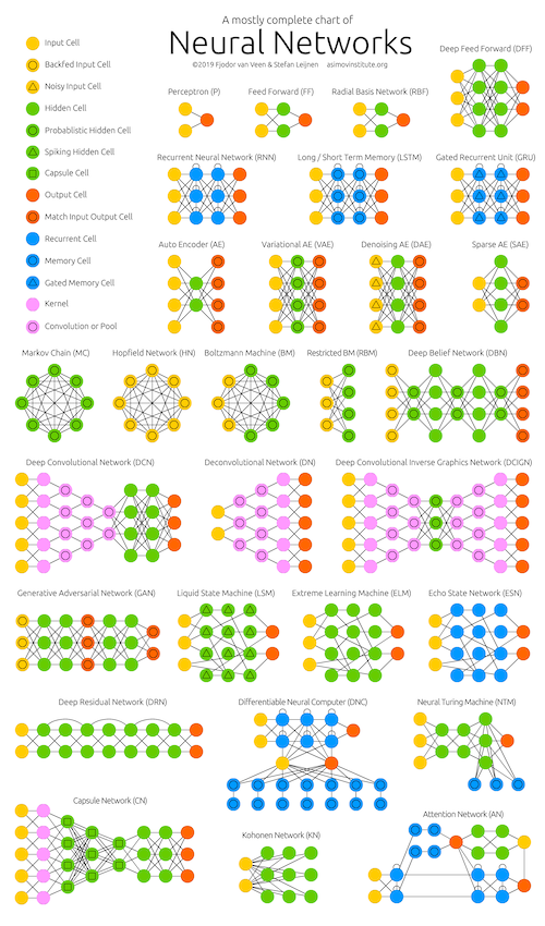
Rockchip has published their own RKNN Model Zoo on GitHub, which captures this in a more practical form. This repo contains pretrained models for a variety of common applications. These models are provided in ONNX format, and can be readily converted to device-specific RKNN weights.
Large Language Models
Support for Large Language Models (LLMs) has been broken out into a separate module called RKNN-LLM. While LLMs are less common in Edge AI applications, this is without doubt the fastest growing area of AI, and deploying LLMs in embedded contexts is an area of active development.
LLMs are still very constrained on devices like the RK3588. RKNN-LLM is mostly in early development and supports small-scale models (e.g., TinyLlama, Qwen-1.8B-Int4). Performance is a far cry from GPT-level performance.
Khadas Resources
Khadas OOWOW
The Edge2 comes built-in with Khadas’ OOWOW service. OOWOW, also known as ‘endless wow’ or infinity wow, is a standalone embedded service for cloud OS installation, device maintenance, and more.
OOWOW will be activated automatically if your device storage is empty, otherwise it can be activated by holding the FUNCTION button while pressing RESET. Once you have configured network access, you will be able to install one of several Android or Linux-based distribution from the cloud!
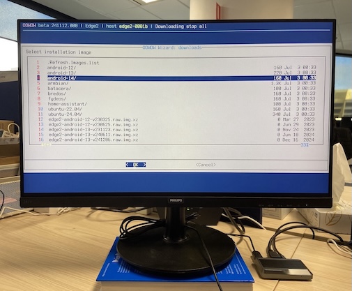
OOWOW Image Selection
Installation only takes a few minutes. Khadas provides documentation and sample code for each platform (Android and Linux), so this is a quick and easy way to get started with the Edge2.
Edge2 Examples
Khadas provides a range of C++ and Python examples for the Edge2, which can be found in the edge2-npu repo on GitHub. This includes C++ and Python examples. The examples all depend on librknn, Rockchip’s custom neural network library. Many of the examples also depend on OpenCV (both C++ and Python).
The C++ examples are much more extensive than those for Python. While there are over ten examples for C++, there are just four for Python.
Quantization
An important part of running a model of the Edge2 is ‘Quantization’ - this is the process by which the precision of model weights is reduced. This can significantly reduce the memory footprint of the model, and ensures that we can take advantage of hardware acceleration available at lower levels of precision. This is typically achieved by applying a ‘scale factor’ that reduces the range of possible values (e.g. -128 to 127 for INT8), then truncating those values to the desired precision.
For example, a model trained with 32-bit floating point (FP32) weights can be quantised to 16-bit floating point (FP16), or even 8-bit integers (INT8), significantly reducing model size and improving inference efficiency, particularly on edge devices.
To learn more about the theory of Quantization, I suggest reading Hugging Face’s Conceptual Guide to Quantization.
Calibration
RKNN Toolkit provides tooling to quantise models while converting them to RKNN format. This not only adjusts the weights, but also adjusts the calculations performed throughout the model to compensate for the scaled down ranges.
Unfortunately, we don’t get this for free. Calibration relies on a selection of sample inputs, which are used to choose the scale factor and zero point values for model weights. The simplest option is Symmetric Quantization, in which the zero point from the original FP range is mapped onto zero in the target (e.g. INT8) range:
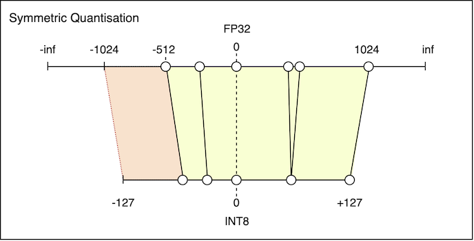
Symmetric Quantization: Notice that some distinct FP values map onto the same INT8 value.
There is also a region of wasted INT8 range on the left.
The reason this is suboptimal is that the minimum and maximum values of the FP range must have the same absolute value. To see why this is wasteful, consider a weight that takes on values from -512 to 1024. Although the true minimum is -512, the range must extend all the way to -1024.
Asymmetric Quantization
Asymmetric Quantization addresses this by allowing the zero point to be shifted to the left, or to the right:
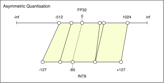
Asymmetric Quantization: Zero point is shifted by -85 units. More of the INT8 range is mapped to positive FP values.
No unused INT8 values on the left.
The key difference here is that the zero point can be chosen as the midpoint between the minimum and maximum FP values. The resulting INT8 range will then cover the entire FP range.
Gotchas
Quantization may seem like a great idea, with very few drawbacks. In practice, it can be hard to track down issues with loss of accuracy, or overall performance of the model. RKNN models are sensitive to input tensor shapes, memory alignment, and batch sizes - these can all impact model performance at runtime.
With YOLOv5 for example, the example code includes some small changes to the underlying model graph. Specifically, a post-processing step is moved outside the main model. This is to address stability issues introduced by quantization.
Datasets
Before we talk about the resources that available for/from Rockchip specifically, it’s worth mentioning some of the datasets that are relevant to Edge AI applications.
MNIST and ImageNet
MNIST and ImageNet are two of the most well known and battle-tested datasets in the field of computer vision models. MNIST is a dataset containing 70,000 grayscale examples of handwritten digits:
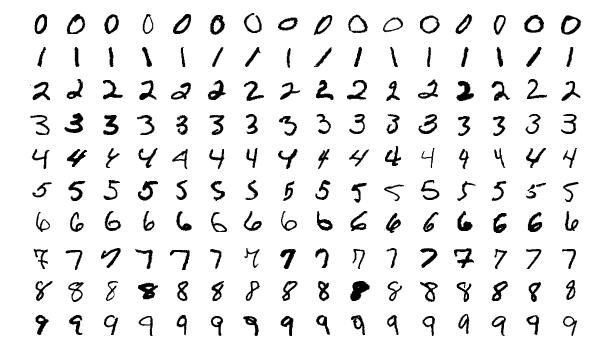
Image Credit: MNIST Examples courtesy of Wikipedia
Performance on MNIST was an important benchmark for early Convolutional Neural Networks (CNNs). Beginning with the ImageNet Large Scale Visual Recognition Challenge in 2012, ImageNet became the defacto standard for measuring performance on image classification tasks. The dataset used for that competition (ImageNet-1K) contains ~1.2 million images, across 1000 classes.
The full ImageNet dataset contains ~14 million labeled images across ~20,000 categories. Although it was created almost 20 years ago, ImageNet continues to be used for training and benchmarking deep learning models on object detection and image classification tasks.
VGGFace2
VGGFace2 is a large-scale face recognition dataset. It consists of ~3.3 million images of ~9100 subjects, downloaded from Google Image Search. The dataset has been designed to capture the variations that arise due to age, socioeconomic background, and the setting in which the images are captured:
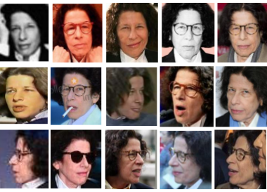
Image credit: Example taken from VGGFace2: A dataset for recognising faces across pose and age.
COCO Dataset
COCO is a large-scale object detection, segmentation, and captioning dataset. It is often used to train and benchmark object detection models, such as YOLO. However the wide range of annotations included in the dataset make it suitable for image segmentation, human pose estimation, and even captioning.
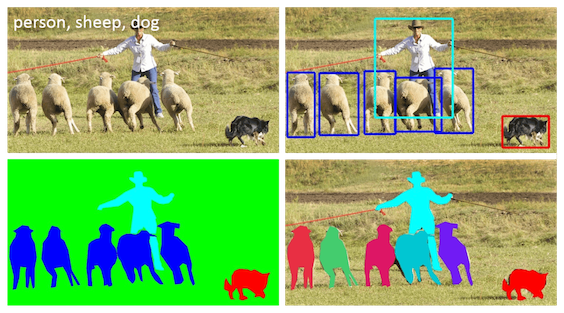
Image credit: Adapted from Figure 1 in Microsoft COCO: Common Objects in Context.
You will often find pretrained object detection models that have been trained on the COCO dataset. COCO defines 91 classes in total, but the dataset only uses 80 of those classes. An off-the-shelf pretrained model will readily categorise objects into one of those 80 classes, and we can use Transfer Learning to re-fit this to our own custom datasets. This is cover in more detail below.
Open Images Dataset
The Open Images Dataset (OID) is another large scale dataset that can be extremely valuable when customising pretrained models. OID contains approximately 9 million images, annotated with image-level labels, object bounding boxes, object segmentation masks, visual relationships, and localised narratives.
The maintainers of OID have partened with Google to offer a tool called FiftyOne that can be used to download subsets of the dataset, as needed for specific tasks. For example, if you wanted to train an object detector to recognise firearms, you could download images (and annotations) for classes such as Handgun, Rifle and Shotgun.
Part 3: Transfer Learning
We now have the fundamental knowledge required to train our own custom object detector. We will take advantage of Transfer Learning, to avoid the cost and complexity of training a model from scratch.
Transfer Learning refers to the practice of using a pretrained model, typical trained on a benchmark dataset like ImageNet or COCO, for a different but related task.
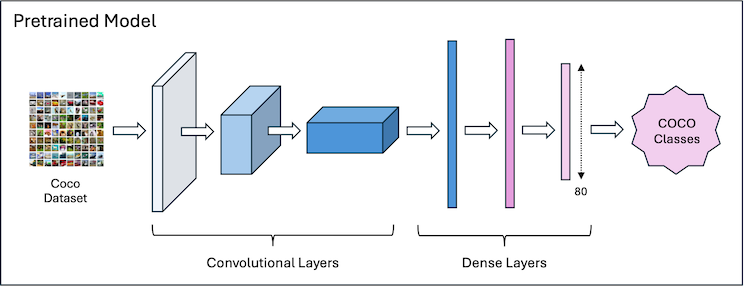
The two main approaches to Transfer Learning are Feature Extraction and Fine-Tuning. These differ in how they treat the existing layers of the model - specifically, whether they are ‘frozen’ or ‘unfrozen’.
Feature Extraction
In Feature Extraction, we freeze all but the top few pretrained layers. Those top layers are then re-trained from scratch, for the new task. This kind of Transfer Learning is very fast, and is well suited to cases where the target task is similar to the original task, or when the target domain is a subset of the original domain.
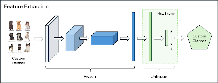
It’s worth nothing that when training a classifier, we will typically replace the topmost layer entirely. If the top layer previously had 80 outputs (e.g. corresponding to the 80 classes in COCO), we would replace that with a new layer, ensuring that the new layer has the number of outputs required for our custom task.
Fine-Tuning
Fine-Tuning takes this a step further. During training, we unfreeze all of the pretrained layers and train them along with the new layers on a custom dataset. Fine-Tuning is more effective when the target dataset is large enough or differs significantly from the original domain.
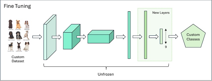
In practice, these two approaches are often combined: training begins with pure Feature Extraction, using frozen pretrained weights. Once the model achieves a reasonable level of performance, the pretrained weights are unfrozen, allowing them to adapt to the new task.
YOLOv5
YOLO, or “You Only Look Once”, is best thought of as a family of object detection models. First introduced in 2015 (original paper here), YOLO has continued to be improved and iterated upon by multiple researchers. You can identify these iterations by a version number suffix (e.g. YOLOv5, YOLOv8, and so on). Many recent advancements have been driven by Ultralytics - an AI company that has built its reputation around pushing the envelope with YOLO object detection.
A deep dive into the implementation details of YOLOv5 is beyond the scope of this post. However, if you would like to learn more, a great starting point is Ultralytics YOLOv5 Architecture.
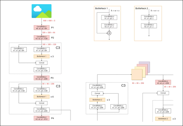
Image credit: A small portion of the YOLOv5 Model Structure from Ultralytics YOLOv5 Architecture.
Source Code
The fastest way to get started with YOLOv5 is via the yolov5 GitHub repo:
# Clone the YOLOv5 repository
git clone https://github.com/ultralytics/yolov5

# Navigate to the cloned directory
cd yolov5

# Install required packages
pip install -r requirements.txt
From here, you can easily run YOLOv5 object detection on your PC. Here are just some of the examples from the yolov5 README file:
# Run inference on a local image file
python detect.py --weights yolov5s.pt --source img.jpg

# Run inference on a local video file
python detect.py --weights yolov5s.pt --source vid.mp4

# Run inference on a screen capture
python detect.py --weights yolov5s.pt --source screen
...
The --weights argument tells detect.py which version of the model to use. There are several to choose from, described below.
There are other scripts in the yolov5 repo that will be of interest to us:
export.py- Exports a YOLOv5 PyTorch model to other formats, e.g. ONNX.train.py- Trains a YOLOv5 model on a custom dataset.
Note that export.py can not export directly to RKNN format. For that, we’ll first need to export a model to ONNX format, then convert that to RKNN format using RKNN Toolkit.
Pretrained Models
Ultralytics provides several pretrained models for YOLOv5. Each is a slightly different variation on the model - larger models have wider layers. The number of parameters is proportional to the Width-Depth Multiple of the model, which scales the number of layers in the model, as well as the width of those layers:
 Model              Width-Depth Multiple   Parameters   Size (MB)   Speed      mAP@0.5 (COCO val)
------------------+----------------------+------------+-----------+----------+-------------------
 yolov5n (nano)     0.25x                       ~1.9M     ~3.9 MB   fastest    ~28.0
 yolov5s (small)    0.33x                       ~7.5M    ~14.0 MB   fast       ~37.4
 yolov5m (medium)   0.67x                      ~21.8M    ~41.0 MB   medium     ~45.4
 yolov5l (large)    1.00x                      ~46.5M    ~92.0 MB   slower     ~49.0
 yolov5x (xlarge)   1.25x                      ~87.7M   ~166.0 MB   slowest    ~50.7
The nano and small variations are well suited to rapid iteration in Edge AI and embedded contexts, where memory and compute are at a premium. However as you can see from the table, this comes at the cost of mAP, or Mean Average Precision. It’s worth digging into this in some detail.
Performance Metrics
For object detection models, the metrics we most care about are Mean Average Precision (mAP) and Intersection over Union (IoU). IoU is best understood in graphical form. Given a ground truth bounding box, and a bounding box prediction, we first calculate the area of the intersection and union of those boxes. We then take the ratio of those two values:
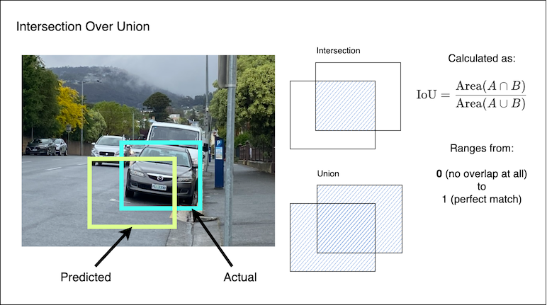
Mean Average Precision is an aggregated metric, that takes IoU into account. Precision answers the question: “Given all the objects the model identified, what proportion of these were actually correct?”
In the results shown above, mAP50 is the Mean Average Precision at IoU = 0.50. This means a prediction is considered correct if its IoU with a ground truth box is at least 0.50.
This measurement can be made stricter and more comprehensive, by averaging the mAP over a range of IoU thresholds. The mAP50-95 metric is the Mean Average Precision averaged over IoU thresholds from 0.50 to 0.95. This is calculated in steps of 0.05 (i.e. 0.50, 0.55, …, 0.90, 0.95).
Head, Neck and Backbone
An important detail of the YOLOv5 model is that it can be separated into three parts:
- The Backbone - This is the main body of the model, responsible for extracting details such as patterns and geometric features.
- The Neck - This takes the information gathered by the backbone, reducing it down by combining and aggregating features.
- The Head - This uses the information aggregated by the neck to make predictions about objects in the image.
This separation allows us to use Transfer Learning to adapt the model to new tasks. We can take advantage of the pretrained Backbone and Neck weights by leaving those frozen - this means they won’t change while we train our custom model. The Head will be replaced with new dense layers, specifically for our custom task. It’s those new layers that will be trained on our custom dataset.
In order to do that, we need to construct an appropriate training dataset.
Building a Dataset
To make the most of Transfer Learning, you need a custom dataset with examples that are representative of a new task. These examples must be annotated using YOLO-style annotations for bounding boxes. The YOLO annotation format is very simple:
<class_id> <x_center> <y_center> <width> <height>
All coordinates are normalized (range 0.0 to 1.0), and the class ID is a numeric index. The advantage of normalized coordinates is that they are independent of a particular image size.
FiftyOne
The Open Images Dataset (discussed earlier) is a great resource for building custom datasets. The OID website provides instructions on how to download a subset of images and corresponding annotations for your task. This includes an open source tool called FiftyOne from Voxel51:
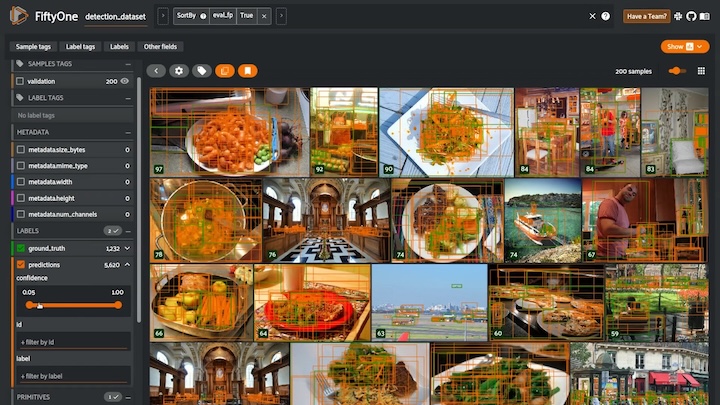
Image Credit: Screenshot from the introductory video included in the FiftyOne Docs
One you have created a custom dataset, you should split it into training, validation and test sets. The training dataset will be used to train the model, while the validation dataset will be used to tweak hyperparameters and to choose a base pretrained model. The test set can be used at the end to evaluate overall performance.
Data Preparation
Since we’re training a YOLOv5 model, we can use train.py from the yolov5 GitHub repo. This distribution contains the latest and greatest that Ultralytics has to offer. To train on a custom dataset, we use the --data argument to provide the path to a YAML file that describes our dataset:
python train.py --img 640 --batch 16 --epochs 20 --data datasets/firearms.yaml
The other arguments here specify the input image size, batch size, and number of training epocs to complete.
There isn’t much to the dataset YAML file, but there is one detail that can be confusing at first:
# this path is relative to the train.py script
path: ../datasets/firearms
train: images/train
test: images/test
val: images/validation

# Classes
names:
  0: Handgun
  1: Rifle
  2: Shotgun
The gotcha here is that path is relative to the train.py script. Let’s say you’ve checked out the YOLOv5 source into a directory called yolov5 and the firearms dataset in a datasets directory alongside that. Printing out the directory tree using tree should look something like this:
% tree . -L 3
.
├── datasets
│   ├── firearms
│   │   ├── images
│   │   └── labels
│   └── firearms.yaml
└── yolov5
    ├── benchmarks.py
    ├── CITATION.cff
    ├── classify
    |
    :   // trimmed for brevity //
    |
    ├── train.py
    └── val.py

22 directories, 61 files
When you set your path, you need to take this directory structure into account.
Training the Model
Training with YOLOv5 will print out heaps of interesting information process about the model, and how it is performing after each epoch.
Assuming you run the same train.py command as above:
python yolov5/train.py \
  --img 640 \
  --batch 16 \
  --epochs 50 \
  --data datasets/firearms.yaml
You should get some output that is similar to this (at the end of the output):
Validating yolov5/runs/train/exp12/weights/best.pt...
Fusing layers...
Model summary: 157 layers, 7018216 parameters, 0 gradients, 15.8 GFLOPs
                 Class     Images  Instances          P          R      mAP50   mAP50-95
                   all         99        129      0.656      0.714      0.722      0.502
               Handgun         99         14      0.677      0.929      0.856      0.687
                 Rifle         99         89      0.824      0.674      0.796      0.532
               Shotgun         99         26      0.467      0.538      0.515      0.287
Results saved to yolov5/runs/train/exp12
The output includes mAP@50 scores for each of the classes in the custom dataset (closer to 1 is better), as well as the mAP@50-95 scores. It’s normal for the mAP@50-95 scores to be lower, since they are stricter and more conservative.
The weights of each run are stored in yolov5/run/trains/exp<run>. You can see above that the output is from run 12, since the path is yolov5/runs/train/exp12. After each run, the best weights will be found in weights/best.pt. This model file is in PyTorch format.
Evaluation
After training, you can evaluate your model using the test set to measure its performance:
python yolov5/val.py \
  --task test \
  --weights yolov5/runs/train/exp12/weights/best.pt \
  --data datasets/firearms.yaml \
  --img 640
The results should look like something like this:
Fusing layers...
Model summary: 157 layers, 7018216 parameters, 0 gradients, 15.8 GFLOPs
                 Class     Images  Instances          P          R      mAP50   mAP50-95
                   all        307        382      0.611       0.57      0.581      0.373
               Handgun        307         57      0.665      0.737      0.698      0.483
                 Rifle        307        259      0.753      0.517      0.677      0.436
               Shotgun        307         66      0.415      0.455      0.368        0.2
Speed: 0.2ms pre-process, 2.8ms inference, 1.7ms NMS per image at shape (32, 3, 640, 640)
Results saved to yolov5/runs/val/exp
Notice there is a reduction in mAP50 and mAP50-95 scores. This tells us that the model does not fully generalise to examples outside of the training dataset. This can indicate the model is over-fitting the dataset.
Conversion
The final step in this process is to prepare the model to run on the Edge2. This requires two conversion steps:
First, we must convert the model from PyTorch to ONNX format. ONNX is a neural network interchange format that is supported as an input format by RKNN Toolkit. This is trivial using the export.py script from Ultralytics YOLOv5:
python yolov5/export.py \
  --data datasets/firearms.yaml \
  --img 640 \
  --include onnx \
  --weights yolov5/runs/train/exp12/weights/best.pt
This will write the ONNX model data to yolov5/runs/train/exp12/weights/best.onnx.
Second, we must convert the model to RKNN format, so that it can run natively on a Rockchip NPU. There are many reasons why a model may not run natively on the NPU (e.g., unsupported layer types, tensor shapes, or memory alignment). This is one of the reasons why it is worth exploring the models in the RKNN Model Zoo.
The conversion to RKNN format is a little more involved, since we need to provide a calibration dataset for quantization. The calibration dataset is simply a subset of images from the full training set, which can be used to estimate zero points and scale factors during quantization.
python3 rknn_model_zoo/examples/yolov5/python/convert.py \
  yolov5/runs/train/exp12/weights/best.onnx \
  firearms-calib.txt \
  rk3588
Closing Thoughts
With native support for INT8/FP16 precision, an efficient NPU, and plenty of examples via RKNN Toolkit, the Rockchip RK3588 offers a well-rounded platform for running real-world AI workloads at the edge. This post has shown that it’s very achieveable to fine-tune and deploy YOLOv5 without needing a server, GPU, or internet connection.
Edge AI is not without its challenges and constraints. As you get further into converting and deploying your own models on the Edge2, you will discover that Machine Learning demands a high level of care. It’s important to invest time in understanding the nuances of quantization, transfer learning, dataset preparation, and evaluation. These are all essential components in an end-to-end inference deployment.
Where to from here?
My hope is that this post inspires you to experiment with some of your own ML models - even without an Edge2, most of what we’ve explored in this post applies to desktop ML too! As for my own experiments, I’m beginning to explore Machine Translation at the Edge, and what is achievable with Tiny Language Models. Stay tuned for that!
References
These are just a handful of references I used while writing up this post. There are many others, and I will update this list as I incorporate feedback.
YOLO:
COCO:
- V7: COCO Dataset: All You Need to Know to Get Started
- Coco dataset, What is it? and How can we use it?
- Papers With Code: COCO (Common Objects in Context)
- Ultralytics: COCO Dataset
Quantization:
- Hugging Face: Quantization
- Maarten Grootendorst: A Visual Guide to Quantization
- Neural Network Distiller: Quantization Algorithms
Floating Point:
ImageNet / ILSVRC: