Sparsehash Internals

One of the C++ topics that have I wanted to write about is Google’s Sparsehash library. Sparsehash provides several hash-map and hash-set implementations, in particular sparse_hash_map and sparse_hash_set, which have been optimised to have a very low memory footprint. This post dives into the details of how this is achieved.

Sparsehash also provides dense_hash_map and dense_hash_set, which have been optimised for speed. However, this post will focus on just the inner workings of the sparse_hash_* class templates.

Contents

• Background
• Getting Started
• Example Code
• Hash Collisions
• Internal Data Structures
• Overhead
• Resizing
• Performance
• Sparsepp
• Wrap-up

Background

Hash tables

A hash map - or more generally, a hash table - is a useful data structure for lookup-intensive applications. It’s primary advantage is that lookup, insertion and deletion operations run in constant time, on average.

The efficiency of a hash table comes from the expectation that items are well distributed across an array that is typically much larger than the number of items it contains. Each location in the array represents a bucket (or slot), with items assigned to a bucket based on the output of a hash function. This array will typically be allocated as a single block of memory.

One drawback to hash tables is that they require more memory than alternative data structures, such as binary trees. This is because when the underlying array becomes too full, the probability of a conflict - where more than one item hashes to the same bucket - will increase. The solution is to make the array large enough, relative to the number of items in the hash table, that the probability of a conflict has a reasonable upper bound.

Sparse arrays

What makes sparse_hash_map clever is that it uses a sparse array to minimise the overhead of empty buckets. A sparse array implementation assumes that a large proportion of the entries in an array are unset, or contain some default value.

A sparse array will usually incur a performance penalty, but through clever bitmap manipulation techniques, Google’s sparse array implementation preserves the constant time complexity of lookup, insertion and deletion operations. However, it is important to recognise that these operations may be slower by a constant factor.

Getting Started

Sparsehash currently lives on GitHub, where you will find both the original implementation and an experimental C++11 version. This code has been released under a BSD-3 license.

Sparsehash has been designed as a header-only library, however packages are also available for various operating systems.

For this example, we will start by cloning the Sparsehash repository, and build/run the test suite:

git clone https://github.com/sparsehash/sparsehash.git
cd sparsehash
./configure
make

Now we can run the tests:

./hashtable_test
./libc_allocator_with_realloc_test
./simple_compat_test
./simple_test
./sparsetable_unittest
./template_util_unittest
./type_traits_unittest

No issues? Then we can proceed to our example program…

Example code

Let’s start with a simple example:

#include <iostream>
#include <string>
#include <sparsehash/sparse_hash_map>

// A sparse_hash_map typedef, for convenience
typedef google::sparse_hash_map<std::string, std::string> MyHashMap;

int main() {
    // Construct a sparse_hash_map
    MyHashMap my_hash_map;
    my_hash_map["roses"] = "red";
    std::cout << my_hash_map["roses"] << std::endl;
    return 0;
}

Assuming you place this code in a file called ‘sparsehash-demo-1.cpp’, one level above your ‘sparsehash’ clone, you could compile and run this using clang:

clang++ sparsehash-demo-1.cpp -I ./sparsehash/src -o sparsehash-demo-1
./sparsehash-demo-1

You can no doubt guess what the output will be:

red

Let’s move on to a more complex example, that will allow us to explore various aspects of the sparse_hash_map API. This example defines a custom value type, and includes a call to an interesting function called set_deleted_key:

#include <algorithm>
#include <iostream>
#include <string>

#include <sparsehash/sparse_hash_map>

// A custom value type that has a default constructor
class MyValueType {
public:
    // The usual boilerplate
    MyValueType() : _value("unknown") {}
    MyValueType(const MyValueType &other) : _value(other._value) {}
    MyValueType(const char *value) : _value(value) {}
    void operator=(const MyValueType &other) {
        _value = other._value;
    }
    const std::string asString() const {
        return _value;
    }
private:
    std::string _value;
};

// Allow value type to be redirected to std::ostream
std::ostream & operator<<(std::ostream &o, const MyValueType &value) {
    o << value.asString();
    return o;
}

// A sparse_hash_map typedef, for convenience
typedef google::sparse_hash_map<std::string, MyValueType> MyHashMap;

int main() {
    MyHashMap my_hash_map;
    my_hash_map.set_deleted_key("");

    my_hash_map["roses"] = "red";

    // The other way to insert items, as with std::map
    const std::pair<MyHashMap::const_iterator, bool> result =
        my_hash_map.insert(std::make_pair("violets", "blue"));
    if (!result.second) {
        std::cout << "Failed to insert item into sparse_hash_map" << std::endl;
        return 1;
    }

    std::cout << "violets: " << result.first->second << std::endl;

    // The other way to retrieve values
    const MyHashMap::iterator itr = my_hash_map.find("violets");
    if (itr == my_hash_map.end()) {
        std::cout << "Failed to find item in sparse_hash_map" << std::endl;
        return 1;
    }

    // Fails if 'set_deleted_key()' has not been called
    my_hash_map.erase(itr);

    // Accessing values using [] is only permitted when the value type has a
    // default constructor. This line will not compile without one.
    const MyValueType &roses = my_hash_map["roses"];

    // Print output
    std::cout << "roses: " << roses << std::endl;
    std::cout << "violets: " << my_hash_map["violets"] << std::endl;

    return 0;
}

Place this in a file called ‘sparsehash-demo-2.cpp’, and compile as before. Running ‘sparsehash-demo-2’ should produce the following output:

violets: blue
roses: red
violets: unknown

The key take-home points here are that a default constructor is required to support the [] accessor, as with std::map.

We can also see that we need to call set_deleted_key before calling erase(), to define a ‘deleted key’. Why is this the case?

The reason comes down to hash collisions.

Hash Collisions

A hash collision occurs when two or more items have the same hash, and therefore map to the same location in the hash table. There are two ways to resolve collisions:

• Closed Addressing
• Open Addressing

Closed Addressing

In Closed Addressing, or separate chaining, a linked list or an array is used to store all of the items that hash to a particular location in the hash table. This resolves the problem of collisions, but can result in an O(n) worst-case lookup time if all keys map to the same location in the array.

Assuming that a linked list is used, there are two ways that we can implement this. The first is using an external linked list, where each location in the array contains a pointer to the head of a linked list. In this scheme each node in the linked list contains a pointer to an item stored in that bucket.

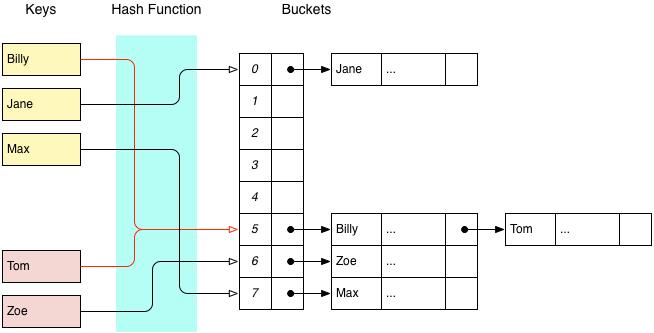
The other approach is to use an internal linked list, where each item maintains a pointer to the next node in the list, and the first item in a bucket is stored directly in the underlying array.

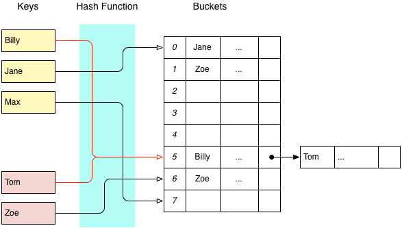
External linked lists tend to have lower memory overhead, since the array only needs to be large enough to store pointers. However, an internal linked list may be desirable when collisions are rare, or when you would like to avoid the cost of pointer indirection.

Open Addressing

The alternative to Closed Addressing is called Open Addressing, and this is what Sparsehash uses. When a key is mapped to a bucket that has already been used, a probing scheme will be used to find another available bucket somewhere else in the array. The simplest probing scheme is linear probing:

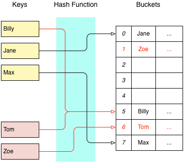
With linear probing, when a collision occurs each successive bucket will be examined to find a place for the new item. The search terminates when an empty bucket is found. Lookups are performed using the same probing scheme. For reasons discussed in your favourite algorithms textbook, Sparsehash uses a technique called quadratic probing to find available buckets, e.g.:

where $x$ is the number of probes so far. This formula gives the following sequence, assuming $i$ is the first bucket identified:

These indices will wrap if they pass the end of the array. When used with a good hash function, this technique ensures that every bucket in the hash table is probed before the same value is produced. However, deleting items may break this chain, and that is why we need a special deleted key - to ensure that future probes do not terminate prematurely.

Internal Data Structures

sparsehashtable

Both sparse_hash_map and sparse_hash_set are implemented using a class template called sparsehashtable. This class template provides all of the functionality needed by a hash table data structure, including hash collision logic and triggers that will resize the table when the load factor becomes too high.

sparsetable

Going one level deeper, there is class template called sparsetable, a sparse array implementation that uses space proportional to the number of elements in the array. This allows a sparsehashtable to have more buckets, while minimising the overhead of empty buckets.

So how does it work?

A sparsehashtable divides an array into groups of 48 elements. Each group is represented as a sparsegroup, which contains an allocation bitmap, a pointer to a data array, and a count of the number of elements that have been set. The allocation bitmap tracks which elements in the group have been assigned, while the data array stores the values for just those elements.

The following diagram illustrates how this works, using a group size of 8 elements for readability. All of the examples and diagrams in this post assume that we are storing a pointer to a record containing a name, and various other data, represented by an ellipsis.

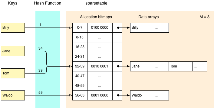
In this diagram each sparsegroup contains 8 buckets, and each bucket contains a pointer to a record. Working from left to right, we can see that the keys ‘Jane’ and ‘Tom’ hash to the values 34 and 39 respectively, so are both located in the 5th sparsegroup. Two bits have been set in the allocation bitmap, corresponding to the 3rd and 8th positions in the data array. The data array contains space for two values - those corresponding to ‘Jane’ and ‘Tom’.

Overhead

Let’s examine Sparsehash’s overhead claims.

When a sparsegroup is first constructed, the allocation bitmap is zeroed out, and the data array pointer will be set to NULL. The memory overhead at this point is 48 bits for the bitmap, and 4 or 8 bytes for the pointer to the data array (depending on whether the code has been compiled to use 32-bit or 64-bit pointers), and 2 bytes to maintain a count of the number of items in a sparsegroup.

Using 32-bit pointers, the raw overhead for an empty sparsegroup, in bits, can be calculated as:

Or 2 bits per bucket.

What happens when a bucket needs to be allocated?

When a bucket is first allocated, a sparsegroup will allocate a data array that is large enough to hold a single item. The allocation bitmap will also be updated so that the relevant bit is set. We can break this down to find the overhead for unused entries.

Let unused_bitmap = 47, unused_data_ptr = 32 / 48 * 47, and unused_counter = 16 / 48 * 47. Then the number of bits that can be attributed to unused entries, is:

Here, the unused_data_ptr and unused_counter terms calculate how much of the cost of those fields can be attributed to unused buckets. When we divide this by the number of unused buckets, the number of bits of overhead per unused bucket works out to be…

Combining the unused_data_ptr and unused_counter terms, and substituting $n$ for 47 this generalises to:

where $n$ is the number of unused buckets. So under this interpretation, unused buckets have 2 bits of overhead when using 32-bit pointers. And for 64-bit pointers:

Allocator overhead

Unfortunately, this isn’t the complete picture. This note, taken from the Sparsehash documentation, explains why:

The numbers above assume that the allocator used doesn’t require extra memory. The default allocator (using malloc/free) typically has some overhead for each allocation. If we assume 16 byte overhead per allocation, the overhead becomes 4.6 bit per array entry (32 bit pointers) or 5.3 bit per array entry (64 bit pointers).

This is assuming 16 bytes (or 128 bits) of overhead per memory allocation for 32-bits pointers, and 32 bytes for for 64-bit pointers.

Resizing

There are two situations in which a hash table may need to be resized - the first being when a table becomes too full, and other being when the table becomes too empty. Most hash table implementations allow these thresholds to be determined via maximum and minimum load factor parameters. The defaults for sparsetable are 0.80 and 0.20, respectively.

One quirk of sparsetable is that deleting items will never result in the table being resized. The table will only ever be resized on the next insert operation, which means that calling ‘erase’ does not invalidate any iterators. This also means that a table could contain a large number of ‘deleted item’ entries. Resizing a table will discard these items, but they are counted towards a table’s load factor when inserting items.

Performance

In general, the performance of a hash table is affected a number of factors:

1. Choice of hash function
2. Distribution of key values
3. Load factor thresholds
4. Resize factor

These are discussed in various robust algorithms texts. But what we’re really interested in is the performance impact of using sparse_hash_map over other map implementations.

Test program

The Sparsehash source code includes a program called ‘time_hash_map’ that will test the performance of sparse_hash_map, dense_hash_map, as well as other map implementations.

Tests are performed in four passes. The first pass will insert 10 million items, with sequential integer keys, and associated objects that are 4 bytes in size. Subsequent passes halve the number of items inserted, but double the size of the associated objects. This is so that maximum memory usage remains constant for different object sizes.

It is not difficult to extend this program to test other map implementations. For each map implementation that should be tested, you need to provide a class template that has a resize() function. Here is the definition for EasyUseSparseHashMap:

// For pointers, we only set the empty key.
template<typename K, typename V, typename H>
class EasyUseSparseHashMap<K*, V, H> : public sparse_hash_map<K*,V,H> {
public:
    EasyUseSparseHashMap() { }
};

Note that the standard hash_map implementation that will be tested is selected when you run configure. To find out which hash_map implementation has been chosen, look for a line similar to the following:

checking the location of hash_map... <unordered_map>

Results

If you built Sparsehash as described earlier in this post, running the ‘time_hash_map’ will produce output with the following structure:

SPARSE_HASH_MAP (4 byte objects, 10000000 iterations):
map_grow              248.0 ns  (23421757 hashes, 53421814 copies)
map_predict/grow      116.6 ns  (10000000 hashes, 40000000 copies)
map_replace            28.2 ns  (10000000 hashes,        0 copies)
map_fetch_random      159.8 ns  (10000000 hashes,        0 copies)
map_fetch_sequential   37.0 ns  (10000000 hashes,        0 copies)
map_fetch_empty        13.1 ns  (       0 hashes,        0 copies)
map_remove             49.6 ns  (10000000 hashes, 10000000 copies)
map_toggle            192.3 ns  (20399999 hashes, 51599996 copies)
map_iterate             6.5 ns  (       0 hashes,        0 copies)

stresshashfunction map_size=256 stride=1: 369.8ns/insertion
stresshashfunction map_size=256 stride=256: 314.3ns/insertion
stresshashfunction map_size=1024 stride=1: 597.1ns/insertion
stresshashfunction map_size=1024 stride=1024: 657.7ns/insertion

This shows the benchmarks for various map operations, as applied to 10 million entries each with a 4 byte value. For comparison, running this on my laptop produces the following results for Google’s dense_hash_map:

map_fetch_random       28.4 ns  (10000000 hashes,        0 copies)
map_fetch_sequential    5.1 ns  (10000000 hashes,        0 copies)
map_fetch_empty         1.2 ns  (       0 hashes,        0 copies)

This is notably faster than the sparse_hash_map results, but YMMV.

Although somewhat dated, the following post contains a comprehensive benchmark of various hash table implementations:

• Big Memory, Part 3.5: Google sparsehash!

Sparsepp

Given the high bar set by Sparsehash, I would be remiss if I did not mention Sparsepp. Inspired by Sparsehash, Gregory Popovitch developed Sparsepp as a faster and more memory-efficient replacement for std::unordered_map. Here is the example from the Sparsepp README file:

#include <iostream>
#include <string>
#include <sparsepp/spp.h>

using spp::sparse_hash_map;

int main()
{
    // Create an unordered_map of three strings (that map to strings)
    sparse_hash_map<std::string, std::string> email =
    {
        { "tom",  "tom@gmail.com"},
        { "jeff", "jk@gmail.com"},
        { "jim",  "jimg@microsoft.com"}
    };

    // Iterate and print keys and values
    for (const auto& n : email)
        std::cout << n.first << "'s email is: " << n.second << "\n";

    // Add a new entry
    email["bill"] = "bg@whatever.com";

    // and print it
    std::cout << "bill's email is: " << email["bill"] << "\n";

    return 0;
}

Sparsepp also boasts better compatibility with C++11, with support for move constructors.

An important difference in Popovitch’s sparse_hash_* implementation is that calling erase() may invalidate iterators. This is because Sparsepp releases memory when items are erased, so setting a ‘deleted key’, while permitted for compatibility, is no longer required.

The Sparsepp repository includes a detailed benchmark and comparison of Sparsepp and Sparsehash with other map implementations. It is worth pointing out that it was Popovitch who noticed the potential impact of allocator overhead, which has since been noted in the Sparsehash documentation.

Popcount

Another interesting difference between Sparsehash and Sparsepp is how a sparsegroup determines the location of an item in the sparsegroup data array. To locate the item at position $i$ in a sparsegroup, we want to count the number 1’s that occur before position $i$ in the bitmap. For example, given a bitmap:

01011001

we would find that the data array index for item 4 (zero-indexed) is 2.

Whereas Sparsehash uses a lookup table, the Sparsepp implementation uses either a native CPU instruction (if available) or an intricate little algorithm, typically known as ‘popcount’:

static size_type _pos_to_offset(group_bm_type bm, size_type pos)
{
    return static_cast<size_type>(spp_popcount(bm & ((static_cast<group_bm_type>(1) << pos) - 1)));
}

The important part here is the call to spp_popcount(), which is delegated to s_spp_popcount_default() when a native CPU instruction is not available:

static inline uint32_t s_spp_popcount_default(uint32_t i) SPP_NOEXCEPT
{
    i = i - ((i >> 1) & 0x55555555);
    i = (i & 0x33333333) + ((i >> 2) & 0x33333333);
    return (((i + (i >> 4)) & 0x0F0F0F0F) * 0x01010101) >> 24;
}

static inline uint32_t s_spp_popcount_default(uint64_t x) SPP_NOEXCEPT
{
    const uint64_t m1  = uint64_t(0x5555555555555555); // binary: 0101...
    const uint64_t m2  = uint64_t(0x3333333333333333); // binary: 00110011..
    const uint64_t m4  = uint64_t(0x0f0f0f0f0f0f0f0f); // binary:  4 zeros,  4 ones ...
    const uint64_t h01 = uint64_t(0x0101010101010101); // the sum of 256 to the power of 0,1,2,3...

    x -= (x >> 1) & m1;             // put count of each 2 bits into those 2 bits
    x = (x & m2) + ((x >> 2) & m2); // put count of each 4 bits into those 4 bits
    x = (x + (x >> 4)) & m4;        // put count of each 8 bits into those 8 bits
    return (x * h01)>>56;           // returns left 8 bits of x + (x<<8) + (x<<16) + (x<<24)+...
}

Hacker’s Delight

How popcount works goes beyond the scope of this post, but if you find these kinds of bit manipulation tricks fascinating, you will enjoy this book:

At time of writing, the author’s website is down, but you can find the 2nd Edition on Amazon.

Wrap-up

As with any choice of data structure in a compute- or memory-constrained environment, you will want to run your own tests to determine which data structure will best suit your needs.

Sparsehash provides hash table implementations that occupy two very different regions in the space of compute/memory trade-offs. But while Sparsehash is obviously battle-hardened, you should consider newer offerings such as Sparsepp, which explore the space further.

And even if you choose to stick with std::unordered_map or even just std::map, having some insight into how alternatives work under-the-hood will help you design tests, and identify potential pitfalls, that will best inform your decision.